This blog post accompanies the SDPB Monday Macro segment that airs on Monday, March 7, 2022. Click here to listen to the segment.

In 1921, Frank Knight (1885 – 1972), preeminent economist and a founding member of the (University of Chicago’s) Chicago School of economic thought, published, while an associate professor of economics at Iowa State University, Risk, Uncertainty and Profit, a 375-page treatise on the role and “peculiar income” of the entrepreneur in a free-enterprise economy (232). In the book, Knight now-famously and painstakingly distinguished between the concepts of risk and uncertainty; the latter, incidentally, is the source of the entrepreneur’s peculiar income—but that’s a topic for another day.

According to Knight (1921), risk is “measurable uncertainty” (233). This is to say, risk is a concept that refers to a distribution of possible outcomes about which we are reasonably well informed, because of theoretical deduction—the probability of rolling a three with a fair, six-sided die is 1/6—or empirical induction—the probability of being struck by lightning is 1/500,000. To use Knight’s (1921) terms, 1/6 is an “a priori” probability, whereas 1/500,000 is a “statistical probability,” and both characterize risk (224-225).

In stark contrast, uncertainty—or, in the parlance of economics, Knightian uncertainty—is a concept that refers to a distribution of possible outcomes about which we know very little, because “there is no valid basis of any kind for classifying instances” (225). As Knight so eloquently explained,

The practical difference between the two categories, risk and uncertainty, is that in the former the distribution of the outcome in a group of instances is known (either through calculation a priori or from statistics of past experience), while in the case of uncertainty this is not true, the reason being in general that it is impossible to form a group of instances, because the situation dealt with is in a high degree unique.

Knight (1921), p. 233; a priori is italicized in original.

These days, the terms risk and uncertainty—of the epidemiological and geopolitical sorts and otherwise—fill the headlines, while the distinction between the two concepts, and their implications for effective macroeconomic policy, fill the thoughts of macroeconomists. This is because risk and uncertainty make designing and implementing macroeconomic policies, such as monetary and fiscal policies, very difficult. And, as you might imagine—and unfortunately for macroeconomic policymakers and the rest of us—of the two concepts, uncertainty is the greatest challenge to effective policymaking these days, when we are dealing with, at the very least, known unknowns, to borrow a now-familiar phrase.

Models, parameters, and timing

In the context of policymaking, risk and, to an extent larger than we often care to countenance, uncertainty broadly describe what economists refer to as the limits of our knowledge; that is, the limits of what we—as policymakers, say—can know about the economy. In addition to (a priori and statistically measurable) risks and (unmeasurable) uncertainties of unforeseeable macroeconomic outcomes, such as the pandemic lockdown, supply-chain disruptions, or labor-market inefficiencies, economists must manage model, parameter, and timing uncertainties. To understand and appreciate the limits imposed by these sorts of uncertainties, consider them in the context of a simple macroeconomic general-equilibrium model, defined as the intersection of aggregate demand and aggregate supply, which I illustrate in Figure 1.

Figure 1: A Macroeconomic Equilibrium Model

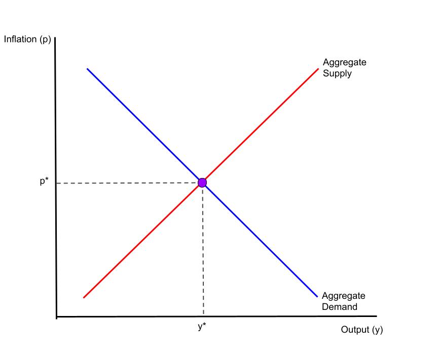
Briefly, and as readers of Schooled know well, in Figure 1, the horizontal axis measures output—think, real GDP—and the vertical axis measures the rate of inflation. The aggregate demand curve reflects the total amount of expenditures demanded by all sectors of the economy: namely, households, firms, governments, and foreign buyers of our goods and services. The aggregate demand curve is downward sloping in this space because, given some growth rate in the quantity of money circulating in the economy, the total amount of expenditures demanded falls [rises] as the inflation rate rises [falls]. The aggregate supply curve reflects the total productive capacity of the economy. The aggregate supply curve is upward sloping in this space because, given the prices and quantities of the inputs to production, total output rises [falls] as the average price level of final goods and services rises [falls]. The intersection of the aggregate demand and aggregate supply curves simultaneously determines the equilibrium rate of inflation (p; vertical axis) and the equilibrium level of output (y; horizontal axis).

According to this model, inflation rises if either the aggregate-demand curve shifts to the right (because consumer confidence rises, for example) or the aggregate-supply curve shifts to the left (because supply chains are disrupted by a pandemic, for example). And, finally, monetary and fiscal policies shift the aggregate demand curve: for example, a contractionary monetary policy, which raises the interest rate, shifts the aggregate-demand curve to the left, lowering inflation and output.

Or so says the model

Model uncertainty refers to specifications of the model, which reflects the limits of our knowledge about how the economy operates. For example, what is the probability the interest rate drives aggregate demand and, thus, output and inflation, in the ways conventional monetary theory predicts in Figure 1? Or, what is the probability the demand for money is proportional to income, so increasing the money supply increases inflation? Or, what is the probability households save deficit-financed tax cuts in anticipation of a future tax hike? A priori, based on some theoretical deduction, we know the answers to these questions are, of course, unknown.

But wait! Perhaps we could infer, based on empirical induction, some basic features of the model’s specifications, such as the parameter value that describes how inflation responds to the interest rate. This is to say, perhaps we could compute, based on our observations of the economy, a statistical (rather than an a priori) probability of what we do not otherwise know. For example, perhaps we could compute, based on past instances of how the economy responded when the central bank raised the interest rate, a probability of how the economy would respond to a higher interest rate today—a timely topic to be sure. Unfortunately, in many, though not all, instances, parameter uncertainty renders this approach to assigning statistical probabilities difficult. This is because, at the very least, assigning a statistical probability requires a sufficient number of suitable observations, so that our parameter estimate is precise enough to allow us to infer something economically meaningful. For example, the sort of precision that would allow us to know that in 66 percent of the times when the central bank raises the interest rate by 1 percent, inflation falls between 2 and 2.5 percent within a year. As you might imagine, the luxury of such precision is exceptionally rare.

And then there is timing uncertainty. In practice, macroeconomic policies are not state contingent: macroeconomic policies cannot reflect the current state of the economy at all times. This is because policies are not typically incremental—rather, the government commits to extend unemployment insurance payments for a number of predetermined weeks, for example—or easily reversible—rather, the central bank is not inclined to raise and, then shortly thereafter, lower the interest rate, because reversing course could highly destabilize the financial system (and introduce policy uncertainty!), for example. And, in any case, macroeconomic policies are susceptible to so-called inside and outside lags. An inside lag is the time between when policymakers identify a macroeconomic problem and when policymakers implement their solution; fiscal policy includes lengthy inside lags, because of the time Congress takes to pass legislated tax changes, for example. An outside lag is the time between when policymakers implement their solution and when it takes effect in the economy; monetary policy includes lengthy outside lags, because of the time a change in the interest rate requires to affect aggregate demand, for example. Consequently, given the non-state contingent nature of macroeconomic policies and the uncertainties around the timing of their effects, a decision not to act (until we know more) could sometimes prove optimal.

Known knowns

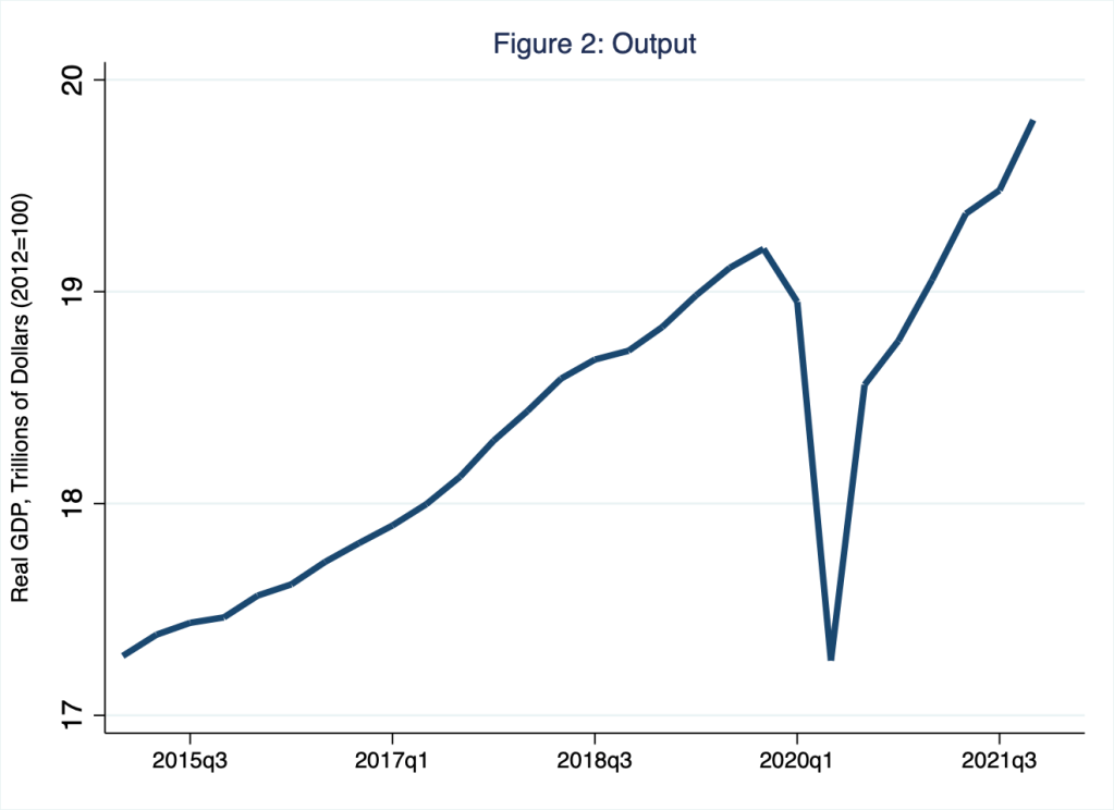
Currently, we live with the macroeconomic consequences of the pandemic, which initially caused output to contract dramatically and suddenly at an annualized rate of roughly 40 percent in the second quarter of 2020. Since then, output has returned relatively quickly to a level roughly consistent with full employment; I illustrate this pattern in Figure 2.

Meanwhile, the rate of inflation has risen substantially, as the services share of consumption expenditures contracted and, consequently, the durable goods and non-durable goods shares of consumption expenditures expanded. Put differently, a few months after the pandemic struck the United States, consumers decreased their expenditures on services such as haircuts and, instead, increased their expenditures on durable goods such as couches and non-durable goods such as toilet tissue. This sudden shift in consumer preferences would have strained supply chains in the best of times; amid a pandemic, the outcome effectively amounted to an aggregate-supply shock (to durable and non-durable goods). In Figure 3, I illustrate this inflationary pressure according to the personal consumption expenditures (PCE) index, the Federal Reserve’s preferred measure of the rate of inflation. (For more on the preference shock the pandemic imposed and the consequences for inflationary pressures, see Monday Macro segment, Habemus Praefectus!)

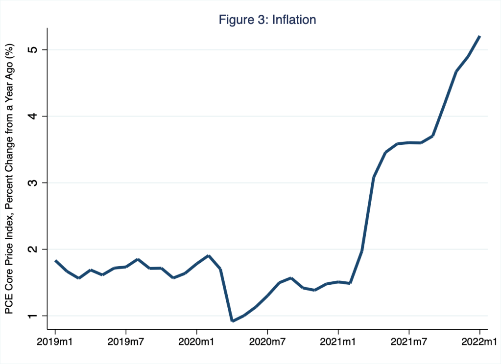
According to Figure 3, in recent months, rates of inflation have landed well outside and above the central bank’s—or anyone else’s—comfort zone. In January 2022, core-PCE inflation registered 5.2 percent. In contrast, the Federal Reserve prefers a sustained annual rate of inflation around 2 percent. Consistent with the supply-shock narrative that I propose here (and several other economists have proposed elsewhere), the greatest inflationary pressures correspond to goods sectors, as opposed to service sectors, of the United States economy. In Figure 4, I illustrate this pattern in the context of the consumer price index (CPI), a measure of the rate of inflation with which the general public is most familiar.

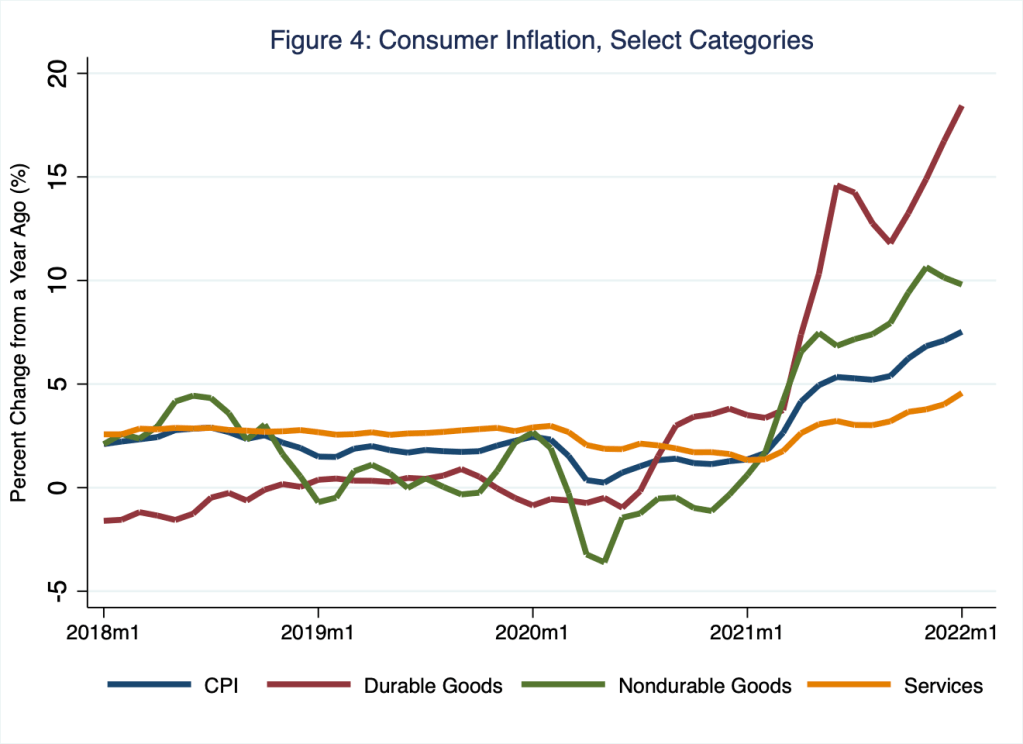
Admittedly, as inflationary pressures persist, and rates of inflation, however we measure them, continue to rise in ways we have not witnessed for several decades, distinctions between goods inflation (red and green lines in Figure 4) versus services inflation (amber line in Figure 4) ring increasingly hollow. The fact of the matter is that the purchasing power of money is falling—relative to all goods and services, including labor services—at unacceptably high rates. Low and stable inflation, what macroeconomists refer to as price stability, is essential in a market economy, in which relative prices—the price of coffee relative to the price of tea or the price of gasoline relative to the price of coal, for example—rightly inform decisions of households, firms, and governments, provided the purchasing power of money is stable. Thus, price stability allows an economy to allocate resources efficiently. Currently, price stability, by any reasonable definition and measure, does not prevail in the United States economy.

Known unknowns: macroeconomic policy under Knightian uncertainty

The supply-chain disruptions the pandemic induced effectively reduced the economy’s ability to produce goods and services all else equal—including monetary policy and the rate of inflation. In the context of our model of a macroeconomic general equilibrium (Figure 1), supply-chain disruptions effectively shifted the aggregate supply curve to the left in the way I illustrate in Figure 5, where the outcome is higher inflation and lower output.

Figure 5: A Macroeconomic Equilibrium Model and a Shift of the Aggregate Supply Curve

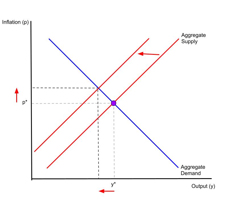
The so-called cost-push inflation that I illustrate in Figure 5 left macroeconomic policymakers with a very difficult choice: return inflation to its original level (p*)—this would require decreasing aggregate demand and further reducing output—or return output to its original level (y*)—this would require increasing aggregate demand and further increasing inflation.

In the immediate wake of the pandemic, amid unprecedented Knightian uncertainties—limits of our knowledge in the contexts of unforeseeable macroeconomic outcomes as well as model, parameter, and timing uncertainties—macroeconomic policymakers chose to stimulate and stabilize output, in part because they underestimated the inflationary consequences of doing so; put differently, the parameter estimates associated with the macroeconomic model specified in Figure 1 were exceptionally imprecise. Moreover, policymakers did not immediately respond to emerging inflationary pressures (around late-summer 2021, for example) because of timing uncertainties: policymakers rightly understood macroeconomic policy to be other than state contingent; because policy is practically irreversible, policymakers waited for more information on the state of the economy before tightening monetary policy.

In recent weeks, the Federal Reserve has made its near-term intentions clear: the central bank intends to tighten monetary policy, because it deems inflationary pressures unacceptably strong. The costs of waiting for more information about the future, the economic models, their parameters, or the optimal timing of macroeconomic policies outweigh the benefits, or so the central bank now estimates based on a distribution of outcomes it cannot know.

Amid Knightian uncertainty, one thing policymakers must know is humility.

References

Knight, Frank H.  1921.  Risk, Uncertainty and Profit. New York: Sentry Press.