This blog post accompanies the SDPB Monday Macro segment that airs on Monday, March 6, 2023. Click to here to listen to the segment, which begins at minute 13:30. And for more macroeconomic analysis, follow @NSMEdirector.

Macroeconomic success has many fathers, macroeconomic failure is an orphan. Policy makers tend to credit their policy decisions and their economic philosophies more generally for high employment or strong personal-income growth, for example. And to be fair, such policy makers often believe their reasoning for assigning such credit; after all, they act as they do because they intend to effect positive economic change, so of course their policies and philosophies have something to do with good economic outcomes that follow—or so the reasoning, which seems fundamental to our human nature, goes. Meanwhile, of course, bad economic outcomes, including high inflation or broken supply chains, must be the outcomes of someone else’s policies and economic philosophies. In reality, individuals—policy makers, presidents, and so on—rarely cause macroeconomic outcomes in intentional, precisely predictable ways. Thus, assigning credit—think, “fathers”—or blame—think, “orphans”—is more difficult than it may first seem. In this blogpost, I consider how best to assign credit or blame for the macroeconomic outcomes since COVID. I begin with a national perspective and then, I consider the case of South Dakota, home of Schooled.

The recession in 2020 was a public-policy orphan.

A freak, epidemiological event, and not a U.S. policy maker, was responsible for the early days of crisis in 2020. This is to say, an aggregate-supply shock induced by COVID buffeted the U.S. (and world) economy, instigating a deep recession in the first and second quarters of 2020. The recession was followed shortly thereafter by expansionary fiscal and monetary policies—CARES Act and near-zero interest rates, for example—that stimulated aggregate demand. And there is no question the combination of a negative aggregate-supply shock and a positive—policy induced—aggregate-demand shock caused the excessive inflation with which we now contend. Nevertheless, some inflation would have very likely occurred in any case, because a negative aggregate-supply shock is fundamentally inflationary; this is to say, a negative aggregate-supply shock causes inflation, independently of whether the government responds with expansionary macroeconomic policy. To see this pattern, consider an aggregate-supply shock, absent an aggregate-demand shock, in the context of a simple macroeconomic general-equilibrium model, defined as the intersection of aggregate demand and aggregate supply, which I depict in Illustration 1.

Illustration 1: Macroeconomic Equilibrium and a Negative Aggregate-Supply Shock

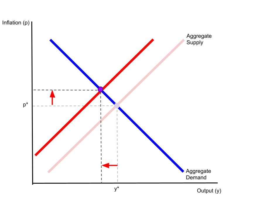
Briefly, and as readers of Schooled know well, in Illustration 1, the horizontal axis measures output—think, real GDP—and the vertical axis measures the rate of inflation. The aggregate-demand curve reflects the total amount of expenditures demanded by all sectors of the economy: namely, households, firms, governments, and foreign buyers of our goods and services. The aggregate-demand curve is downward sloping in this space because, given some growth rate in the quantity of money circulating in the economy, the total amount of expenditures demanded falls [rises] as the inflation rate rises [falls]. The aggregate-supply curve reflects the total productive capacity of the economy. The aggregate-supply curve is upward sloping in this space because, given the prices and quantities of the inputs to production, total output rises [falls] as the average price level of final goods and services rises [falls]. The intersection of the aggregate-demand and aggregate-supply curves simultaneously determines the equilibrium rate of inflation (; vertical axis) and the equilibrium level of output (; horizontal axis).

According to this model, inflation rises if either the aggregate-demand curve shifts to the right (because consumer confidence rises, for example) or the aggregate-supply curve shifts to the left (because of a pandemic, for example). And finally, monetary and fiscal policies also shift the aggregate-demand curve: for example, an expansionary fiscal policy, which increases transfer—think, stimulus—payments, and monetary policy, which lowers interest rates, shifts the aggregate-demand curve to the right, raising inflation and output.

During COVID, an aggregate-supply shock instigated inflation by effectively reducing the economy’s ability to produce goods and services all else—including the supply of money—equal. This is to say, in the context of our model of a macroeconomic general equilibrium, the aggregate-supply curve shifted to the left in the way I depict in Illustration 1, raising inflation and lowering output; the outcome was inflation combined with recession.

One way to detect the inflationary consequences of the aggregate-supply shock is to decompose the corresponding consumer-price inflation into goods, which are generally dependent on manufacturing supply chains and desired during a work-from-home craze, and services, which are less so. In figure 1, I illustrate this decomposition, which I measure on the vertical axis in percentage changes from a year ago; the growth of durable-goods prices appears in dark red.

According to Figure 1, the average price level of durable goods—and to a lesser extent, nondurable goods—rose the most during the worst of the supply-chain crisis. And importantly, the average price level of durable goods rose late in the first half of 2020, before macroeconomic stimulus entered the economy; this is to say, the negative aggregate-supply shock alone caused the prices of durable goods to rise, expansionary macroeconomic policy had not been implemented yet. Interestingly, as the supply-chain crisis has ebbed, the average price level of durable goods has grown more slowly; the last data point in Figure 1 is negative: the average price level of durable goods has fallen recently.

The excessive inflation post 2020 has two fathers, whom economists could forgive to some extent.

In principle, inflation combined with recession imposes on macroeconomic policymakers a very difficult choice: return inflation to its original level (; Illustration 1)—this requires decreasing aggregate demand and further reducing output; in the parlance of macroeconomics, destroying demand—or return output to its original level (; Illustration 1)—this requires increasing aggregate demand and further increasing inflation. In practice, recession imposes on policymakers another problem: how to determine full employment, the maximum level of output the economy could produce without creating price pressures. During COVID, policymakers—fiscal and monetary “fathers”—responded to the COVID-induced aggregate-supply shock with good intentions. Policy makers chose to increase aggregate demand and further increase inflation. They implemented expansionary macroeconomic policies knowing they did not know precisely the level of full employment, which, in hindsight, they apparently overestimated.

Consequently, despite the excessive inflation it currently experiences, the U.S. economy has very nearly achieved a level of output consistent with in Illustration 1; this is to say, actual output has nearly achieved its potential level. Thus, the real economy—the economy we measure in terms of output, labor, capacity utilization, and so forth—seems quite strong, a macroeconomic feature of the U.S. economy that we could discern regionally as well, including for example in the state of South Dakota.

To see the effects of macroeconomic stimulus—and, thus, the macroeconomic expansion post (COVID-induced) recession—on households in the nation and in the region, consider personal income per capita in the U.S. and in South Dakota, which I illustrate in Figure 2.

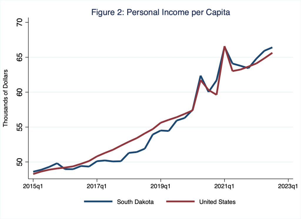
Three observations regarding Figure 2 are particularly noteworthy: personal income per capita in the nation and in the region have increased since 2015, the macroeconomic stimulus—and, thus, the expansion post (COVID-induced) recession—significantly increased personal income per capita during the pandemic and the attending deep recession (thanks to stimulus payments to households), and personal income per capita in South Dakota is currently above personal income per capita in the U.S.; this last observation is evident in Figure 2, where the blue line (South Dakota) rises above the red line (U.S.) in the most-recent quarters.

The current high-performing real economy is an estranged child—not quite orphan—of policy.

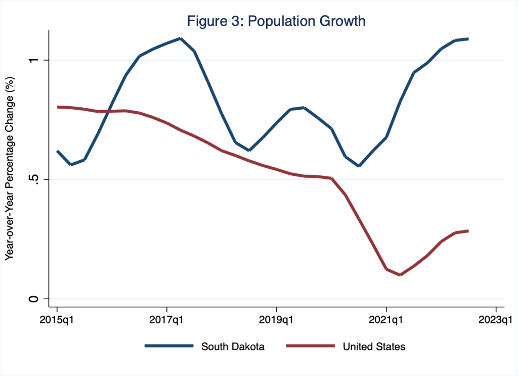
Why personal income per capita is relatively high in South Dakota is a bit complicated, as is assigning credit for this good economic outcome. And to be sure, personal income per capita in South Dakota has performed exceedingly well—this is to say, better than Figure 2 implies—because, as I illustrate in Figure 3, population growth in the state has far exceeded population growth in the nation; recall, personal income per capita is personal income divided by the population, which is growing faster for South Dakota than for the nation.

To understand what is going on, and if anyone can reasonably take credit for the very good economic outcomes in the state, consider the following simple decomposition of personal income per capita.

According to this decomposition, personal income per capita—on the left side of the equals sign in the expression—is equal to labor productivity times the employment rate times the labor-force participation rate . Thus, labor productivity, the employment rate (or, one minus the unemployment rate), and the labor-force participation rate drive personal income per capita. And so these drivers must explain why personal income per capita in South Dakota is greater than personal income per capita in the U.S.

In Figure 4, I illustrate the employment rate for South Dakota and the nation.

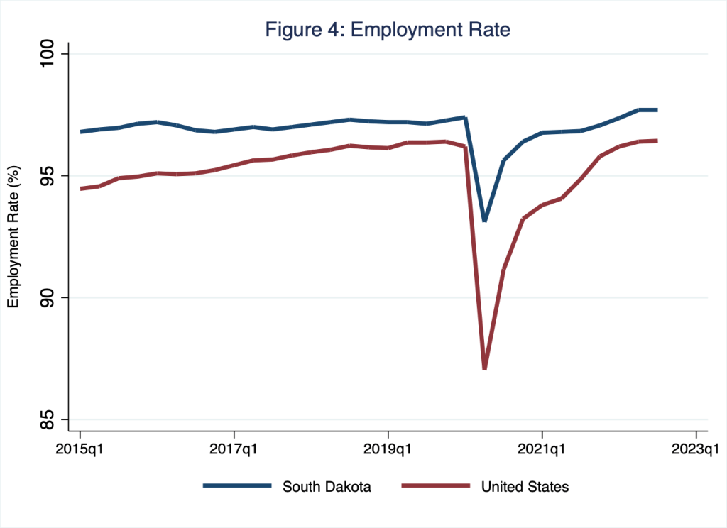
According to Figure 4, the employment rate in South Dakota has consistently outperformed the employment rate in the nation; or, put differently, the unemployment rate in South Dakota has remained below the unemployment rate in the nation. So then, one reason why personal income per capita is relatively high in South Dakota is that the employment rate is relatively high in South Dakota. Next, in Figure 5, I illustrate the labor-force participation rate for South Dakota and the nation.

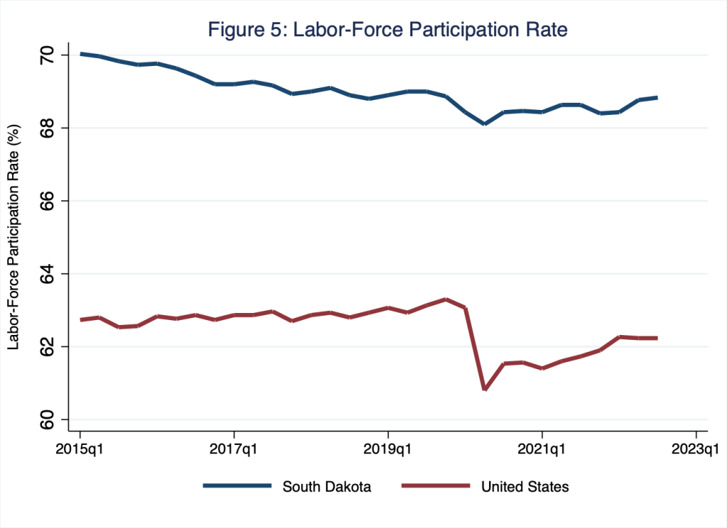
According to Figure 5, the labor-force participation rate in South Dakota has consistently outperformed the labor-force participation rate in the nation; or, put differently, a relatively large share of the working-age population in South Dakota is either employed or actively seeking employment. Moreover, unlike in the U.S. overall, the labor-force participation rate in South Dakota did not fall persistently after COVID. So then, another reason why personal income per capita is relatively high in South Dakota is that the labor-force participation rate is relatively high in South Dakota.

Finally, the third driver of personal income per capita is, of course, labor productivity , which, in any quarter, is implied by the values of personal income per capita, the employment rate , and the labor-force participation rate according to the arithmetic expression above. This is to say, if we know personal income per capita, the employment rate, the labor-force participation rate, and the arithmetic expression above, we could roughly estimate labor productivity. Consider, for example, Table 1, in which I decompose personal income per capita in the third quarter of 2022 into these three drivers.

Table 1: Personal Income per Capita Decomposition, 2022:Q3

	Personal Income per Capita	Labor Productivity	Employment Rate	Labor-Force Participation Rate
South Dakota	$66,413	$98,755	0.98	0.69
United States	$65,636	$109,368	0.96	0.62

According to Table 1, in the third quarter of 2022, personal income per capita in South Dakota ($66,413) was greater than personal income per capita in the United States ($65,636), because the employment rate in South Dakota (0.98) and the labor-force participation rate in South Dakota (0.69) were relatively high; even though, labor productivity in South Dakota ($98,755) was below labor productivity in the United States ($109,368). Put another way, average personal income in South Dakota is relatively high because labor markets in the state are relatively tight (and have been since long before COVID).

The exceptionally tight labor markets in South Dakota post COVID have been driven, in part, by COVID-era expansionary macroeconomic policies, which introduced an exceptionally large amount of fiscal stimulus into the state while interest rates remained near the zero lower bound (throughout the nation, of course). Meanwhile, on balance, expansionary macroeconomic policies and tensions abroad—specifically, in Ukraine—have proven boons to financial and agricultural industries, respectively; these industries are responsible for relatively large shares of state GDP in South Dakota. Thus, the current relative strength of the South Dakota economy has much to do with larger macroeconomic and global forces. Granted, the legal and political environments in South Dakota—think, tax laws and a deregulatory mindset, for example—tend to favor private-enterprise-derived economic outcomes and, thus, private-sector economic growth. However, these environments, many of which economists tend to applaud, are not new; rather they have been around since long before COVID. Put another way, assigning credit for the recent, relatively high personal income per capita in South Dakota is not entirely straightforward; nevertheless, the primary drivers seem to be broad based, associated mostly with domestic-macroeconomic and global forces.

Of course, despite the story of a tight labor market in which employers are competing vigorously for a limited supply of employees, particularly in South Dakota, households are not experiencing a rise in purchasing power in return for their labor services. In Figure 6, I illustrate the year-over-year percentage change in real personal income per capita, which measures the year-over-year percentage change in the purchasing power of (nominal) personal income per capita.

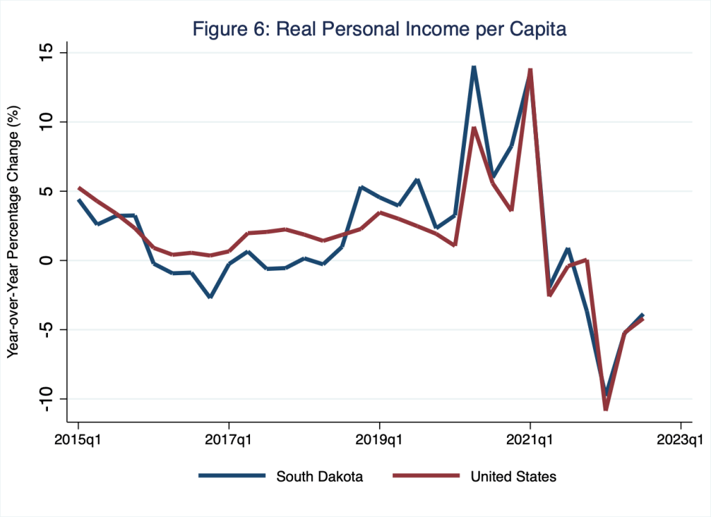
According to Figure 6, households in South Dakota and beyond are losing purchasing power, because inflation is eroding their household income.

While we could forgive policy makers for crediting their policy decisions and their economic philosophies more generally for good economic outcomes, and for disassociating themselves with bad economic outcomes, identifying cause and effect in macroeconomic policy is difficult work. Perhaps the most important takeaway from our current macroeconomic circumstances is that this is no time to argue about taking credit or assigning blame. As I illustrate in Figure 6 and explain in greater detail in Poorhouses, household budgetary positions are deteriorating. It’s time for sensible macroeconomic policy, no matter its parent.