This blog post accompanies the SDPB Monday Macro segment that airs on Monday, June 5, 2023. Click here to listen to the segment. For more macroeconomic analysis, follow J. M. Santos on Twitter @NSMEdirector.

During the pandemic, the supply of money in the United States rose dramatically, reaching 27 percent year-over-year growth in February 2021. However, since December 2022, the supply of money has been shrinking, thanks in part to the ongoing contractionary monetary policy the Federal Reserve has implemented since the pandemic. In Figure I, I demonstrate this rollercoaster pattern of exceptionally-high and, then, exceptionally-low growth in the supply of money; I take as my measure of money, M2, which includes currency and coins held by the non-bank public, checkable deposits, travelers’ checks, savings deposits, time deposits under $100,000, and shares in retail money market mutual funds—or, as I like to tell my students, the stuff with which you could buy lunch at Jimmy Johns, for the most part.

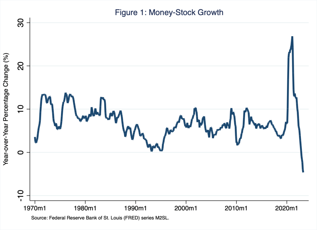
According to Figure 1, the growth of the supply of money during and after the pandemic has been, like every other macroeconomic feature of the pandemic, extraordinary. At no time since 1970, has the supply of money grown as much or as little as it has grown in the last three and half years or so. As I argued in a recent Schooled post, It’s Only Money, although the rates of inflation with which the U.S. and world economies currently contend were instigated, in part, by supply (chain) shocks, inflation is ultimately a monetary phenomenon: the outcome of too much money chasing too few goods—supply-chain constrained or otherwise. To see this relationship between the supply of money and the rate of inflation, consider Figure 2, in which I illustrate the growth in the supply of money—the blue line I illustrate for a longer time period in Figure 1—and the rate of inflation—the red line, based on the personal consumption expenditures core price index—from just before the pandemic to now.

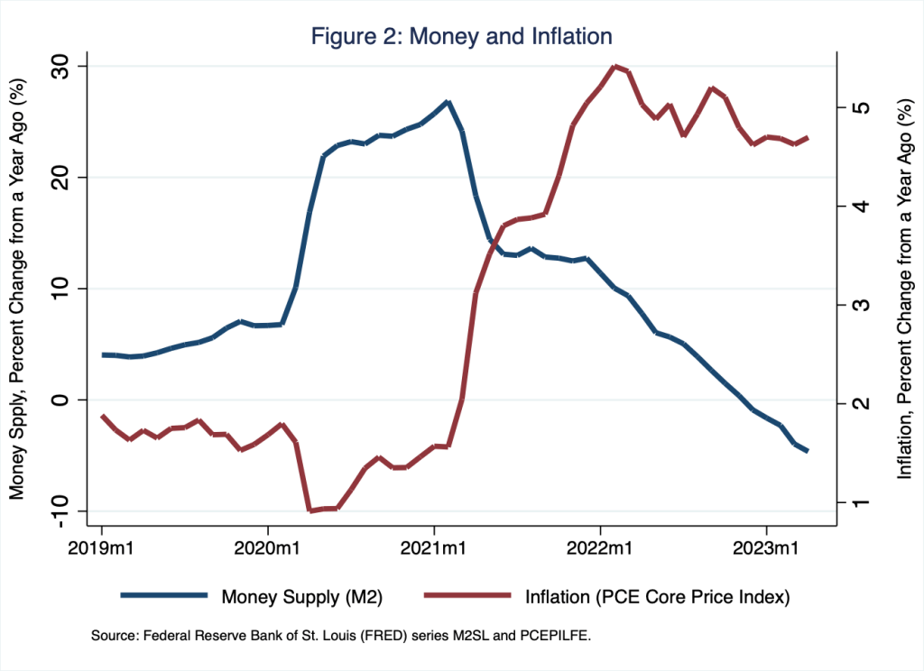
According to Figure 2, the exceptional growth in the supply of money preceded by about one year the exceptional growth in the rate of inflation; this one-year-long lag between the growth rate of the supply of money and the rate of inflation is typical: most estimates of the lag, which can vary from inflationary episode to inflationary episode of course, fall within 12 to 18 months.

A closer inspection of Figure 2 reveals something even more interesting, though. At the start of 2021, the growth in the supply of money fell precipitously, returning to a plateau just above 10 percent near the start of 2022; and since then, the growth of the supply of money has fallen steadily. Meanwhile, the rate of inflation has remained stubbornly in the neighborhood of 5 percent. Put differently, although the growth of the supply of money has been falling for well over a year, the rate of inflation has not budged. Reasoning as we do that the growth of the supply of money is the principal driver of the rate of inflation, what explains the seeming disconnect between the current growth of the supply of money and the current rate of inflation?

Enter a rather obscure monetary concept macroeconomists refer to as velocity.

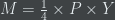
Velocity is the average number of times the supply of money is exchanged to purchase goods and services over time. As it happens, for the last several months, the velocity of money has risen—a pattern that is inflationary, all else equal. To understand how specifically the supply of money, its velocity, and the rate of inflation are related, consider the following quantity equation, which Schooled readers have no doubt seen before.

In this equation, represents the supply of money, represents the income velocity of money, represents the average price level, and represents real income, which economists typically measure as real Gross Domestic Product (GDP); thus, is nominal GDP. Velocity is a crucial feature of the quantity equation and the relationship between the supply of money and the rate of inflation more generally.

In terms of the quantity equation above, velocity is the average number of times the supply of money is exchanged to purchase nominal income . To define velocity arithmetically, then, rearrange the quantity equation as follows.

For example, suppose the supply of money in the economy is $50 ; and during a year in the economy, 100 pencils are produced, purchased, and valued at a price of $2 each so that . In this example, the income velocity of money equals 4 times per year : $50 of money pays for $200 of nominal income per year, because each dollar in the supply of money is exchanged on average 4 times per year:

Setting aside real GDP for now, the quantity equation explains how the flow of the supply of money affects the flow of nominal income and, possibly, the rate of inflation, provided we assume why individuals hold—or, in the parlance of monetary economics, demand—money, as opposed to illiquid assets such as real estate or equity shares in corporations, the stuff with which you could not buy lunch at Jimmy Johns. Assume, as economists often do for simplicity, individuals hold money in fixed proportion to their nominal income, so the velocity of money is constant over time. In the example above, where , the fixed proportion would be 0.25, the reciprocal of 4: because each dollar in the supply of money is exchanged on average 4 times per year to purchase nominal GDP , in money-market equilibrium (where the demand for money equals the supply of money), the demand for money equals 0.25 times nominal GDP. To arrive at this conclusion, rearrange the quantity equation as follows.

Put differently, then, in equilibrium, the velocity of money reflects individuals’ preferences to hold money in relation to the goods and services individuals wish to purchase with money: in the example above, individuals prefer to hold, on average, an amount of money equal to 25 percent of nominal GDP: for example, if nominal GDP equals $20 trillion, the amount of individuals’ wealth they collectively prefer to hold as money is $5 trillion. Relatively low velocity—think, is small—implies relatively high demand for money—think, is large. Thus, velocity is not an instrument of monetary policy, something the central bank could easily control or precisely target; rather, velocity reflects our preferences to hold monetary assets—more on the implications of this statement in just a bit.

Finally, a portion of the percentage change in nominal income is reliably driven by non-monetary forces including changes in physical capital, human capital, the labor force, and innovation—long-run features of the macroeconomy. Conceptually, controlling for the effects of these non-monetary forces on nominal income isolates the effects of the supply of money and velocity on the average price level: all else equal, the supply of money determines the average price level; or put differently, the growth in the supply of money is the principal cause of the rate of inflation. In Table 1, I demonstrate the strength of this relationship in the case of the U.S. economy over the last several decades.

Table 1: Quantity Equation: The U.S. Experience

Time Period	M	V	P	Y
1960 – 2019	1.7%	-0.1%	0.8%	0.8%
1960 – 1979	2.0%	0.1%	1.1%	1.0%
1980 – 1999	1.4%	0.2%	0.8%	0.8%
2000 – 2019	1.5%	-0.5%	0.5%	0.5%
2021 – 2023	1.2%	1.0%	1.5%	08%

For each time period to which I refer in Table 1, I report the average quarterly growth rates of the supply of money , velocity , the price level , and real GDP . According to the quantity equation, the growth rate of the supply of money plus the growth rate of velocity equals the rate of inflation plus the growth rate of real GDP. This is to say:

where we read, “” as “percentage change in.” Informally, if times equals times , then the percentage change in plus the percentage change in equals the percentage change in plus the percentage change in ; we have mathematics, not macroeconomics, to thank for this multiplicative-to-additive property (which is most accurate when the percentage changes are very small—on the order of a few percentage points at most).

In the context of Table 1, then, in each row, the sum of the first two numbers should equal (save some rounding errors) the sum of the last two numbers. Consider, for example, the time period 1960 – 1979: the percentage change in plus the percentage change in equals 2.1% (2.0% + 0.1%), and the percentage change in plus the percentage change in equals 2.1% (1.1% + 1.0%) as well.

With the exception of the last row in the table, high [low] rates of growth of the supply of money tend to correspond to high [low] rates of inflation: for the time period 1960 – 1979, the rate of growth of the supply of money was relatively high (2.0%) and so too was the rate of inflation (1.1%); whereas, for the time period 2000 – 2019, the rate of growth of the supply of money was relatively low (1.5%) and so too was the rate of inflation (0.5%). Meanwhile, velocity remained relatively constant—its growth rate remained near zero.

In striking contrast, the last row in the table reveals a very different pattern: for the time period 2021 – 2023 (Q1), the growth rate of the supply of money was relatively low—the lowest measure of money growth in the table—and the rate of inflation was relatively high—the highest measure of inflation in the table. The reason for the disconnect is the relatively high growth of velocity, which registered an average quarterly growth rate of 1.0%—the highest measure of velocity growth in the table. In Figure 3, I illustrate velocity beginning in 1980.

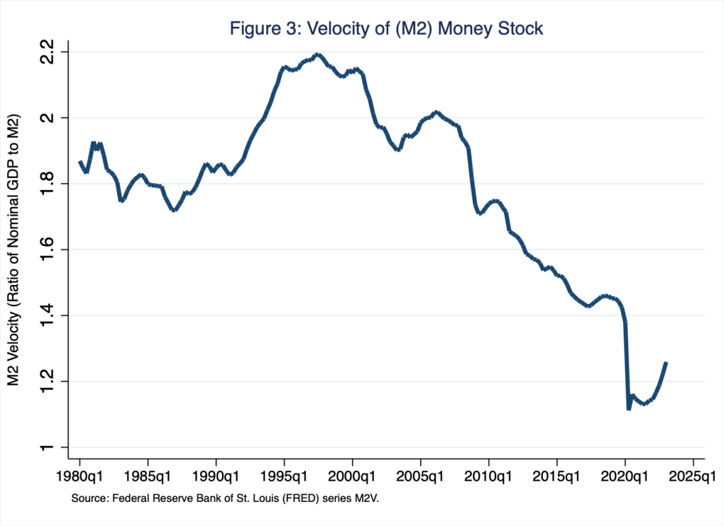
From 1980 to the financial crisis that began in 2008, velocity hovered around 2: each dollar in the supply of money was exchanged on average about 2 times per year to purchase nominal GDP; and thus the demand for money equaled about 0.50 (the reciprocal of 2) times nominal GDP. Velocity fell in the wake of the financial crisis, when “cash was king” and, thus, the demand for money rose. The pandemic accelerated this pattern. In early 2020, velocity hovered around 1: each dollar in the supply of money was exchanged on average about once per year to purchase nominal GDP; and thus the demand for money equaled about 1 (the reciprocal of 1) times nominal GDP. Because velocity was so low during and immediately after the pandemic, the extraordinary growth of the supply of money drove the rate of inflation to “only” about 5 percent (based on the personal consumption expenditures core price index).

As the measure of the growth of velocity I report in the last row of Table 1 suggests, in the last few quarters—far right side of Figure 3—velocity has risen rather suddenly. In the first quarter of 2023, velocity registered 1.3, roughly equal to the value velocity registered in the first quarter of 2020. In the years leading up to the pandemic, velocity registered about 1.5. Thus, if velocity continues to rise quickly, so that the average quarterly growth rate of velocity—the measure I report in the column labeled “V” of Table 1—remains relatively high, then a shrinking supply of money may not lower the rate of inflation: the rate of inflation could remain elevated because the flow of continues to grow at a relatively high rate even though the growth rate of the supply of money continues to fall.

Rising velocity complicates the Federal Reserve’s attempts to reduce the rate of inflation. This is because velocity is fundamentally driven by preferences about how much money we hold as a share of income and how much money we hold in relation to nominal interest rates—the opportunity costs of holding money, which does not earn much, if any, interest. Thus, velocity is not a monetary policy instrument the Federal Reserve can control or precisely target. This is to say, the central bank cannot easily motivate individuals to hold relatively large or relatively small money balances. If anything, currently rising nominal interest rates, a consequence of tightening monetary policy, is causing velocity to rise.

Constant or falling velocity—constant or increasing demand for money—would support the central bank’s efforts to lower the rate of inflation. Unfortunately, individuals seem to prefer otherwise.