This blog post accompanies the SDPB Monday Macro segment that airs on Tuesday, September 5, 2023. Click here to listen to the segment. For more macroeconomic analysis, follow J. M. Santos on Twitter @NSMEdirector.

Long-term interest rates—so-called yields to maturity—are rising, raising the cost of financing for the U.S. government, which finances its expenditures less its tax revenues with the proceeds it collects from selling U.S. Treasury bonds, and everyone else. A bond is a certificate of indebtedness, a so-called IOU, that a borrower sells to a saver; the saver buys the bond—think, lends funds to the borrower—in return for a yield to maturity.  In Figure 1, I illustrate the yield to maturity on a U.S. Treasury bond maturing in ten years (blue line) and the yield to maturity on the average conventional mortgage maturing in thirty years (green line).

In August 2023, the ten-year U.S. Treasury and thirty-year conventional fixed-rate mortgage yields registered 4.17 and 7.07 percent. The last time the ten-year U.S. Treasury yield exceeded 4.17 percent was October 2007, just prior to the global financial crisis; meanwhile, the last time the mortgage yield exceeded 7.07 percent was July 2001, over twenty years ago. In any case, because investors throughout the global financial system reason the U.S. Treasury poses little-to-no material risk of default, the yields to maturity—think, rewards—on U.S. Treasury bonds are consistently lower than yields to maturity on other debt instruments, including the average conventional, thirty-year fixed-rate mortgage. Put differently, then, as yields to maturity on U.S. Treasury bonds rise, so too do yields on all other debt instruments. Thus, the fiscal discipline—fiscal maturity—of the federal government shapes the cost of borrowing more generally, a point to which I’ll return later in this post.

What’s in a yield?

To understand why a long-term yield to maturity—on a Treasury bond or otherwise—rises, decompose the yield into its principal components. The most common way to think about a long-term yield to maturity is the expectation theory, which rests on the efficient-market hypothesis: market-clearing prices—in this case, yields to maturity—sensibly reflect all available information. According to the expectations theory, traders’ expectations of future short-term interest rates determine whether investors buy short-term bonds—and, thus, earn the prevailing short-term yield to maturity—or long-term bonds——and, thus, earn the prevailing long-term yield to maturity; and traders formulate unbiased expectations of the future: traders commit expectation (or forecast) errors, just not in a systematic—think, predictable—way. Traders are rational, not clairvoyant. To understand what the expectations theory of the long-term yield to maturity implies about its composition, consider the following simple—but powerful—example.

Assume for simplicity, a one-year investment horizon is short term and a two-year investment horizon is long term. At the start of period 1, all traders wish to invest $1 for two years; and, to do so, traders may take one of two approaches. Traders may invest $1 for two years—long term in this simple example—and earn in each of the two years the long-term annual yield, , which traders know at the start of period 1. In this case, the gross return at the start of period 1 on the long-term investment approach is the following.

Or traders may invest $1 for one year—short term in this simple example—and earn in that first year the annual yield, , which traders know at the start of period 1; then traders reinvest the proceeds for another year and earn in that second year the annual yield of , which traders do not know at the start of period 1: at the start of period 1, traders must formulate an expectation () about . In this case, the gross return at the start of period 1 on the short-term investment approach is the following.

Because bond traders use all available information in a sensible way, and long-term and short-term investment approaches are simultaneously available, traders’ collective expectation of must be such that, at the start of period 1, . If not, then only the investment approach with the unambiguously higher return would be available; no one in their right mind would take the investment approach with the unambiguously lower return. This efficient-market-hypothesis argument implies the long-term yield to maturity— in my simple example—and the short-term yield to maturity— in my simple example—are related in the following way.

This is to say, the long-term yield to maturity () is the average of current and expected-future short-term yields to maturity ( and , respectively).

For example, suppose the current short-term yield to maturity, , equals 2 percent and the expected-future short-term yield to maturity, , equals 4 percent; put differently, suppose today’s one-year yield to maturity is 2 percent and suppose we expect next year’s one-year yield to maturity to be 4 percent. According to the expectations theory, then, the current long-term yield to maturity, , equals 3 percent, because 3 is the average of 2 and 4. I use yields to one-year and two-year maturities; but the relationship generalizes for longer terms to maturities: in general, a long-term yield to maturity—think, the yield on a U.S. Treasury bond maturing in ten years or the yield on the average conventional mortgage maturing in thirty years—is the average of current and expected-future short-term yields associated with the investment.

Thus, according to the expectations theory, rising long-term yields to maturity generally imply the market expects future short-term yields to rise on average. Finally, economists often slightly modify the prior expression by adding a so-called term premium, , in the following way.

The term premium, $lambda \left(\lambda\right)$, is the additional yield to maturity investors demand because, all else equal (including the path of expected-future short-term rates), investors prefer to buy short-term bonds instead of long-term bonds. In plain English, investors need an additional percentage-point incentive, represented here by , in order to surrender their savings for relatively long periods of time. Sound familiar? It should: our preference to keep as opposed to surrender our savings seems fundamental to human nature.

Lastly, the yield to maturity is a nominal interest rate. Thus, according to the Fisher Effect, the (nominal) yield to maturity is the sum of the real interest rate—the rate at which the lender earns purchasing power on the principal she surrenders to the borrower—plus the expected inflation rate. (For more on the Fisher Effect, see Monday Macro segment, “Gone Fishin’.”) In this way, a yield to maturity—think, in the simple example above, , , and —is the sum of the real interest rate and the expected inflation rate.

Long story short

According to the expectations theory, which we augment with a theory of time preference , and the Fisher Effect, a long-term yield to maturity—think, for example, 7.07 percent, the yield to maturity on the average conventional mortgage maturing in thirty years—is determined by:

1. The expected path of the short-term interest rate—think, , for example—which is the sum of a real interest rate and an expected inflation rate.
2. The term premium—think, .
3. The default premium.

Let’s consider each of these determinants in turn.

The real interest rate. In principle, over time the real interest rate approaches its equilibrium level, what economists refer to r-star (because we denote it, ). is (counterfactually speaking) the “real [inflation-adjusted] short-term interest rate consistent with output equaling its natural rate and constant inflation” (Holston, Laubach, and Williams, 2016). Less formally speaking, is the appropriate real short-term interest rate for a so-called Goldilocks macroeconomy—one that is neither too hot nor too cold but rather just right. Our macroeconomy is approaching “just right” from a place of “too hot,” so likely has more to rise. (For more on , see Monday Macro segment, “R-Star Is Born” and “Stargazing.”)

The expected inflation rate. As the Federal Reserve has tightened monetary policy, the rate of inflation has fallen. For example, according to the consumer price index, the rate of inflation registered 3.3 percent in July. As the rate of inflation has fallen, so too has the rate of expected inflation. In Figure 2, I illustrate three measures of the rate of expected inflation; expectations at the five- and ten-year forecast horizons now register close to 2 percent, the central bank’s target rate.

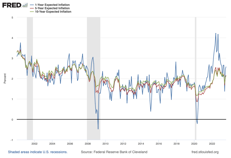
Given the Federal Reserve is seemingly determined to slow the rate of inflation and, thus, the recent path of expected inflation I illustrate in Figure 2, the expected inflation rate is not likely to drive long-term yields to maturity higher anytime soon.

The term premium. The additional yield to maturity—the premium—investors demand because, all else equal (including the path of expected-future short-term rates), investors prefer to surrender their savings for relatively short instead of relatively long periods of time, is a function of investors’ time preference—think, the amount an investor must be paid to consumer later instead of now. Time preference is probably time invariant: the amount an investor must be paid to lend money for two years instead of one year probably does not change much over time. Thus, the term premium is not likely to drive long-term yields to maturity higher anytime soon.

The default premium. Investors are risk averse: all else equal (including the yield to maturity), investors prefer to expose their wealth to less risk. Thus, as default risk rises, the default premium—the amount investors must be paid to expose their wealth to risk—rises as well. There is little to no evidence that default risk on privately issued debt is substantially higher now than a year or two ago. Nevertheless, the political theater surrounding U.S. Treasury debt ceilings and federal government shut downs, coupled with a Treasury debt downgrade issued by Fitch, a bond rating agency, which cited as reason for its downgrade an “erosion of [federal] governance,” and the relatively large federal debt (Figure 3), may be contributing to the rise in U.S. Treasury yields that I illustrate in Figure 1. In Figure 3, I illustrate the federal debt held by the public as a share of GDP; recall, the U.S. Treasury issues federal debt in the form of U.S. Treasury securities, including those that mature in ten years (Figure 1), for example.

According to Figure 3, the federal debt outstanding is roughly the size of the U.S. economy: the share illustrated on the far right of Figure 3 is roughly equal to 100. Meanwhile, the deficit, which is the annual flow that adds to the stock of debt outstanding, is rising (in absolute value). In Figure 4, I illustrate the federal deficit, which registered $1.3 trillion in fiscal year 2022.

And the fiscal position of the federal government has not improved since: as of July 2023, ten months into fiscal year 2023, the deficit measured $1.6 trillion, on path to exceed $2 trillion by the end of this fiscal year (on September 30)—poor fiscal outcomes that reflect the “erosion of governance” to which the Fitch rating agency referred.

Weak federal budgetary and debt positions and rising Treasury yields to maturity make for a vicious cycle: weak federal budgetary and debt positions raise yields to maturity on otherwise-default-free U.S. Treasury bonds; in turn, higher yields to maturity raise federal government expenditures on interest payments on the federal debt. In Figure 5, I illustrate federal government expenditures on interest payments, which are rising in levels (blue line) and as a share of total federal government expenditures (green dashed line).

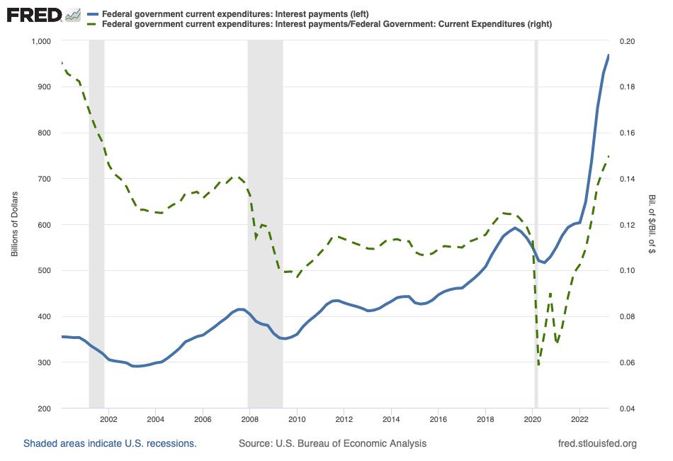
Rising interest payments raise the deficit (in absolute value) and, over time, the debt, further weakening federal budgetary and debt positions. And the path of the vicious cycle is not limited to U.S. Treasury markets, of course, because as yields to maturity on U.S. Treasury bonds rise, yields on all other debt instruments rise as well.

In summary, then, long-term interest rates—yields to maturity—are rising because the long-run equilibrium real interest rate is rising, actual and expected rates of inflation remain elevated, and federal budgetary and debt positions are weakening. Nevertheless, to the extent the current rise in long-term interest rates reflects a return to normal in U.S. credit markets, where I imagine the equilibrium real interest rate must be higher than the levels recorded for much of the period since the global financial crisis, higher long-term interest rates are not necessarily a sign of trouble for the U.S. economy, which has experienced exceptionally—and I would argue, abnormally—low interest rates for too long.

References

Holston, Kathryn, Thomas Laubach, John C. Williams.  2016. “Measuring the Natural Rate of Interest: International Trends and Determinants.”  Federal Reserve Bank of San Francisco Working Paper 2016-11.