This blog post accompanies the SDPR Morning Macro segment that aired Monday, March 11.

In 1900, L. Frank Baum, a denizen, for a time, of Aberdeen, South Dakota, published, The Wonderful Wizard of Oz, a magnificent tale that Metro-Goldwyn-Mayer made into an unforgettable cult classic.  As every child knows, the tale is actually a deeply informed treatise of political and economic controversy surrounding inflationary macroeconomic policy at the turn of the twentieth century, when Populists—including, for the most part, farmers—argued for a bimetallic (silver and gold), as opposed to a monometallic (gold), monetary standard.

Okay, maybe not every child.

In a widely read contribution to the Journal of Political Economy,  Hugh Rockoff (1990) convincingly demonstrates that Dorothy, the embodiment of wholesome middle America, and her fellow travelers—Scarecrow (farmers), the Tin Woodman (industrial workers), and Cowardly Lion (William Jennings Bryan)—travelled to Oz (D.C. and, yes, the abbreviation for ounces, as in ounces of gold) along a monometallic yellow brick road in order to lobby for a bimetallic monetary standard.  Their objective was, in effect, to grow the money supply and, thus, raise the overall price level.  For much of the late nineteenth century, when Baum had come of age, the U.S. economy was mired in deflation, a persistent fall in the overall price level that, in the event, likely repressed U.S. economic growth.  Leaving aside the mechanics of long-gone commodity-money standards such as monometallism and bimetallism, this late-nineteenth century controversy centered on inflation, a phenomenon that remains a subject of U.S. economic and political discourse.

Economists typically define inflation as a persistent, annual rise in the overall price level.  Or, put another way, inflation describes a persistent, annual fall in the purchasing power of money.  This second way of thinking about inflation—that is, thinking about price in terms of the amount of money we exchange for goods and services—rightly emphasizes that, in principle, inflation simultaneously raises the prices of all goods and services by the same proportion; so, in principle, inflation does not change relative prices—the price of mustard (p_m) relative to the price of ketchup (p_k), or p_m/p_k, for example.  A one percent fall in the purchasing power of money simultaneously raises both the price of mustard and the price of ketchup by one percent, leaving p_m/p_k unchanged.  Thus, as Economics Nobel laureate Milton Friedman (1912-2006) tirelessly emphasized, inflation is a monetary phenomenon: over time, the quantity of money drives its purchasing power.

A useful way to think about this relationship between the quantity of money and its purchasing power—a way, incidentally, that Bryan and other Populists likely thought about it—is with the so-called income version of the quantity equation (or, quantity equation, for short), which we specify in the following way.

M × V = P × Y

In this equation, M represents the quantity of money; V represents the income velocity of money; P represents the overall price level; and Y represents real income, which economists empirically measure with real GDP.  The income velocity of money (V) is the average number of times the quantity of money (M) is exchanged for nominal GDP (P×Y), which is valued in units of money.  (For more on real and nominal GDP, see the Morning Macro segment, “Measurement Error.”)  For example, suppose the quantity of money in the economy is $15 (M = $15); and, suppose that during one year 30 pencils are produced and valued at a price of $1 each (P × Y = $30).  In this example, the income velocity of money equals 2: that is, $15 of money facilitates $30 of income per year; each dollar changes hands, on average, 2 times per year in order to purchase $30 of nominal GDP.

The quantity equation is an identity: it is true given how we define M, V, P, and Y.  It does not belong to a particular school of economic thought; for example, both monetarists (like Milton Friedman) and non-monetarists accept the quantity equation.  Nor is it specific about how the quantity of money (M) affects the overall price level (P).  (Algebraically, this lack of specificity is no surprise; the equation includes three unknown variables, assuming the government sets M.)  In order to pin down how the quantity of money affects the overall price level, we need at least a theory for why individuals hold—or, in the parlance of economics, demand—money as opposed to illiquid assets such as homes or ownership shares in corporations.

A useful simplifying assumption is that each individual holds money—a generally accepted means of payment—so she can purchase goods and services, which her nominal income affords.  More specifically, assume each individual holds $1 of money for every $5 of nominal income she earns.  In this case, we specify the demand for money in the economy in the following way.

M = 0.20 × P × Y

Where, again, P × Y is nominal income.  As we assumed, according to this equation, if nominal income is $5, then the individual holds $1 of money (M = 0.20 × $5) so she can purchase goods and services.  Notice, in this economy where individuals hold $1 of money for every $5 of nominal income, each dollar changes hands, on average, 5 times per year; thus, the income velocity of money is equal to 5.  (Or, more technically, solving the quantity equation—think, money-supply equation—and the money-demand equation simultaneously yields an income velocity of money equal to 5, or 1/0.20.)  For our purpose of explaining how the quantity of money affects the overall price level, the important implication of this simplified money-demand theory is that the income velocity of money is constant over time—in this example, V = 5.  (In reality, velocity is not constant; but, assuming it is leads us to the essential features of the actual long-run relationship between the quantity of money and the price level.) 

This framework—the quantity equation combined with a theory of a constant income velocity of money—implies that the quantity of money determines the price level when the economy is operating at full employment.  (At less than full employment, when production capacity is not fully utilized, money may determine real income as well.)  The intuition for this implication is very straightforward: Suppose the money supply suddenly increases once and for all.  All else equal, the demand for money is unchanged, because nominal income (P × Y) is, for the moment, unchanged (and the demand for money is proportional to nominal income); thus, an excess supply of money suddenly exists.  Every individual attempts to trade off her excess supply of money in order to rebalance her wealth portfolio of money versus illiquid assets.  For the economy as a whole, these attempts prove futile—to whom would every individual trade off her excess supply of money?  Thus, the purchasing power of money falls, and the overall price level rises, until money demand again equals money supply.

The quantity theory of money is a very useful way to think about how the quantity of money affects the overall price level and, over time, inflation.  The most convincing examples from history are the least subtle: consider, for example, the hyperinflation that currently plagues Venezuela thanks, in large part, to reckless money creation.  Of course, no matter how we explain what causes inflation, we must measure it empirically; and doing so is a challenge.  This is in part because, in practice, inflationary forces do not simultaneously raise the prices of all goods and services by the same proportion.  (Thus, late-nineteenth century farmers reasoned inflationary forces might raise commodity prices before all others.)  In reality, most firms are imperfectly competitive price setters—as opposed to perfectly competitive price takers—that change their prices infrequently relative to the frequency of inflationary (and microeconomic-market) forces that buffet the economy.  Think, for example, how relatively infrequently a restaurant changes the prices on its menu.  This means our empirical measure of inflation depends on the goods-and-services prices and quantities we choose to sample.

Perhaps the most popular empirical measure of inflation—there are several—is based on the consumer price index (CPI).  In the United States, the Bureau of Labor Statistics (BLS) computes and reports on the CPI each month.  In order to compute the index, the BLS measures, over time, total consumer expenditure on a basket of goods and services that a typical consumer purchases; the BLS surveys households to develop its profile of the typical consumer.  The basket of goods and services is fixed to a BLS-chosen base year.  For each year, the index is the ratio of total consumer expenditure on the basket of goods in services in that year divided by total consumer expenditure in the base year.  Economists measure the inflation rate as the annual growth rate in this index.  In Figure 1, I illustrate U.S. CPI inflation based on the BLS’s broadest basket of goods and services; other measures of the CPI exclude prices of some items, such as food and energy for example.

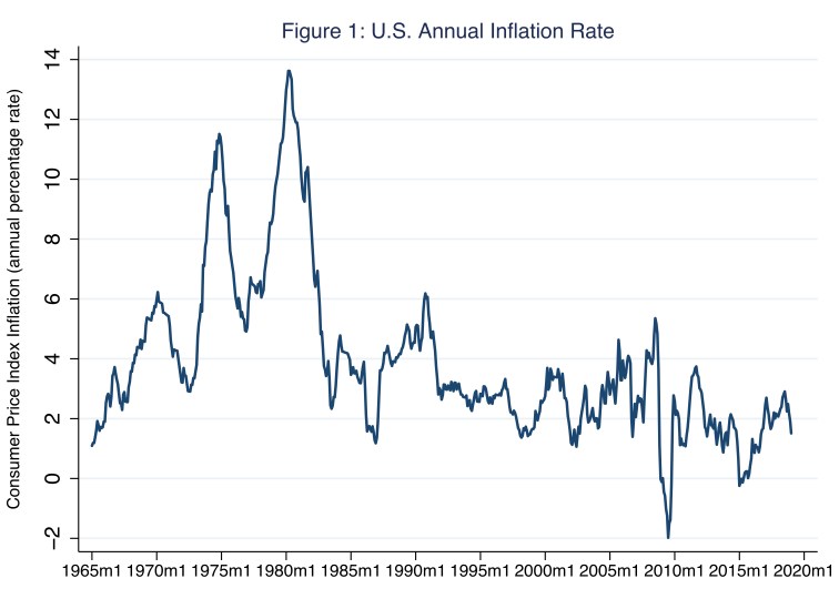
The most striking feature of Figure 1 is the relatively high inflation rates we observe in the 1970s and early 1980s, an episode of U.S. monetary history we call the Great Inflation for obvious reasons.  Consider, for example, early 1980, when the the annual (CPI) inflation rate reached about 13.6 percent.  At that rate, the purchasing power of money loses half its value, and so the overall price level doubles, about every five years.  As you might imagine, economists debate what caused the Great Inflation.  Though, most agree on two aspects of the episode: the rise in oil prices spurred by OPEC cannot adequately explain the persistent inflation; and, in any case, monetary policy was loose—essentially, the money supply increased rapidly.  For example, Athanasios Orphanides (2003) argues that during the Great Inflation the Federal Reserve set interest rates according to a rule designed to drive real GDP to its potential level, which the central bank systematically overestimated, keeping interest rates too low for too long and, thus, fueling inflation.

Since 1990, the annual inflation rate has averaged about 2.4 percent.  At that rate, the purchasing power of money loses half its value, and so the overall price level doubles, about every thirty years, far slower than the doubling rate the overall price level would have achieved had the Great Inflation persisted.  (Incidentally, the Great Inflation did not persist, because discretionary monetary policy tightened—and, consequently, the U.S. economy severely contracted—in the early 1980s.)  Meanwhile, since 1990, the annual inflation rate has deviated quite a bit: in late 1990, the inflation rate was about 6.2 percent; whereas in mid 2009—in the depths of the Great Recession—the inflation rate briefly approached negative 2 percent.  When episodes of negative inflation rates persist, economists term the phenomenon deflation.  Currently, the annual inflation rate hovers slightly below the level monetary policymakers generally prefer.

So, is inflation poisonous or not?  For most economists, the answer depends on the dose.

At the very least, money is an asset that depreciates at the rate of inflation; so, inflation effectively taxes our holdings of money.  More practically speaking, because inflationary forces typically do not simultaneously raise the prices of all goods and services by the same proportion, inflation disrupts economic activity, which depends on a stable price system: prices should move relative to one another because of the microeconomic market forces of supply and demand, not because of macroeconomic changes in the purchasing power of money.  Worse yet, if inflationary forces are volatile, as they tend to be when inflation rates are relatively high, the disruption to economic activity is greater still; hyperinflation is pernicious.  Moreover, inflationary forces discourage buyers and sellers from entering into long-term contracts, an institutional arrangement on which robust economic growth relies.  The problem is that prices set by long-term contracts do not adjust to unanticipated inflation, which capriciously redistributes income between parties to the contract.

Consider, for example, the long-term contractual relationship between lenders and borrowers.  In Figure 2, I illustrate nominal and real interest rates on U.S. Treasury bonds with a maturity of one year; lenders buy these bonds from the U.S. Treasury, the borrower in this case.

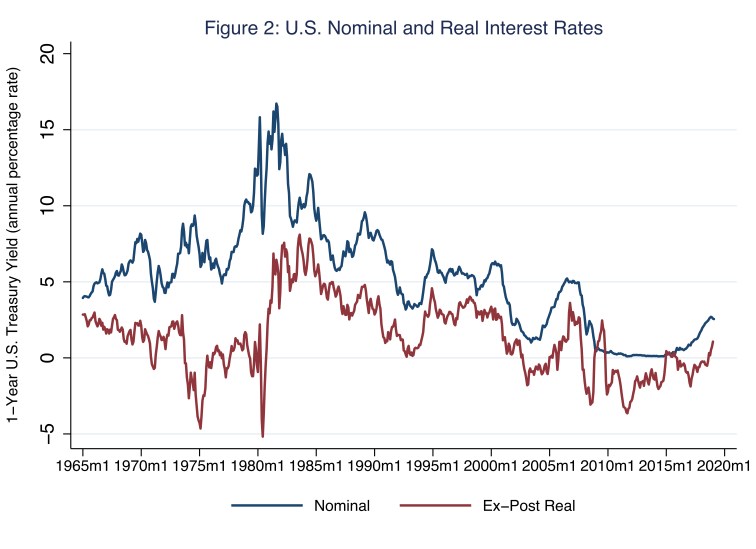
The nominal interest rate is the stated yield to maturity of the bond.  The real interest rate is the nominal interest rate minus the rate of inflation.  As such, the nominal interest rate measures the return to lenders in terms of dollars, whereas the real interest rate measures the return in terms of (real) purchasing power.  The difference between nominal and real interest rates—the vertical distance between blue and red lines in Figure 2—is the inflation rate, ex post in this example.  All else equal, inflation reduces the real return to lenders, thus redistributing income from lenders to borrowers.  (In this way, late-nineteenth century farmers who financed their operations with debt reasoned inflation would lower the real burden of their debt, if only in the short run.)  Consider the path of real interest rates during the Great Inflation when nominal interest rates rose less than one-for-one with the rate of inflation.  During such episodes, the real interest rate fell; when the real rate turned negative, lenders paid borrowers in terms of purchasing power, an outcome lenders surely did not intend or wish to repeat.  This is why nominal and, thus, real interest rates eventually rose, attracting lenders back to the market.

The passage of the Gold Standard Act in 1900 firmly footed the United States on the yellow brick road.  Alas, the Populists did not get the bimetallic standard they sought; though, shortly after the turn of the twentieth century, the overall price level rose thanks, in part, to gold inflows that effectively grew the money supply.  Today the United States abides by a fiat monetary standard: the purchasing power of the U.S. dollar is not linked by statute to a quantity of a commodity such as gold.  Nevertheless, the desire for relative price stability shared by proponents of the gold standard remains generally popular with economists.  On balance, economists recommend a low and stable rate of inflation around 2 percent.  For example, the Federal Reserve sets its inflation target at 2 percent based, incidentally, on the personal consumption expenditures index rather than the CPI.  Essentially, a gradually rising overall price level avoids deflation and encourages long-term contracts reliably indexed to low and stable inflation, thus fueling robust economic growth.  

Additional References

Santos, Joseph M.  2017.  “Monetarism.”  The American Middle Class: An Economic Encyclopedia of Progress and Poverty (Santa Barbara, CA: ABC-CLIO Greenwood), edited by Robert S. Rycroft, pp. 235–239.