This blog post accompanies the SDPR Morning Macro segment that airs on Monday, March 30.

This post draws on research conducted in the Ness School of Management and Economics by Kailie S. Drescher, a graduate student and Dykhouse Fellow who is writing her master’s thesis on the effects of heterogeneous U.S. state-level economic performance on intergenerational mobility.  Figures 1 through 6 and the data analyses required to produced them are thanks to Kailie.

Last Friday, President Donald Trump signed a fiscal-stimulus bill that will inject over $2 trillion into the now-ailing U.S. economy.  The size and scope of the bill are unprecedentedly large.  The bill includes, in part, direct payments to households, loans and grants to businesses, financial support for health-care providers, and transfers to states.  Meanwhile, throughout last week, the Federal Reserve announced its own emergency measures, including lending facilities to financial markets and, possibly, state and local governments.  The extent of these fiscal and monetary policies are appropriate and, in all likelihood, just a start.  By all accounts, the economic impact of the novel coronavirus will be on an order of magnitude of the economic impact of the Great Recession.  In the third week of March alone, 3.28 million individuals applied for unemployment benefits; in the prior (typical) week, just 282 thousand individuals had done so.  And, although the source of the current economic shock is, by the standards of U.S. macroeconomic history, unique, the disruption it will impose on macroeconomic activity will follow two basic, well-worn patterns, the first of which is well understood and appreciated, the second not so much.

First, aggregate economic activity will fall and unemployment will rise in much less time than either measure will require to recover from the shock—so, the easiest way to save economic activity and jobs is not to lose them in the first place.  Second, and far less appreciated, each of the fifty states will experience the downturn and the recovery differently, and in some cases, these differences will be dramatic—so macroeconomic policy must reflect this heterogenous state-level economic performance.  And so it is to this heterogeneity that we now turn.

We like to say that macroeconomists study the economy as a whole.  This is to say, macroeconomists study the general features of the economy: aggregate production (think, GDP and its components), employment, the purchasing power of money (think inflation), and the time value of money (think, interest rates).  (For more on the general features of a macroeconomy, see Morning Macro segments, “Measurement Error,” “Separation Anxiety,” “Follow the Yellow Brick Road,” and “Yield Ahead.”)  To put the matter somewhat differently, macroeconomists tend to abstract from the diversity—or, in economics speak, heterogeneity—of households, firms, and the goods and factor markets—labor and capital markets, for example—in which these households and firms engage.  As a first pass, at least, macroeconomists tend to think about the interactions of so-called representative households and representative firms; these entities represent the interactions of their identical—or, in economics speak, homogeneous—counterparts.

Consider, for example, how macroeconomists tend to think about—and, so, talk about—aggregate production and employment.  In the case of aggregate production, we focus on GDP and its components, and how these measures change over time.  Typically, we decompose real GDP into a trend—which reflects the long-run, regular growth in real GDP—and a business cycle—which reflects the short-run, irregular fluctuations in real GDP.  The expansion phase of the business cycle, which the U.S. economy will surely soon exit, is one of four so-called phases; the other three are peak, contraction (aka, recession), and trough.  (For more on business cycles, see Morning Macro segment, “Growing Old(er).”)  By definition, we observe the business cycle throughout the economy; so, for example, a decline in automobile manufacturing, hospitality services, or economic activity in a specific state, like Alabama or South Dakota, does not, on its own, constitute a contraction.

Likewise, in the case of the labor market, we often cite the unemployment rate in the aggregate: 3.5 percent of the labor force is involuntarily out of work, say.  Where, according to the Bureau of Labor Statistics (BLS), an unemployed individual is anyone who, during the four weeks preceding the BLS survey, was actively seeking employment or waiting to return to work due to a layoff.  By contrast, the BLS defines an employed individual as a paid employee—full or part time, voluntarily or otherwise—or an unpaid employee in a family business.  From what sorts of jobs the unemployed individuals were separated or where these unemployed individuals worked in the United States is not front of the macroeconomist’s mind.  Of course we delve into such details, for which we have lots of data, when we wish to inspect a specific labor-market outcome more deeply; nevertheless, we tend to focus, at least initially, on the most general features of the labor market.  This tendency in the context of the labor market and all other general features of the macroeconomy leads macroeconomists to homogenize, in effect, the U.S. economic experience, which, of course, is not the same for everyone living in the U.S. economy.  In this blog post, we showcase the diversity of state-level economic experiences over the business cycle.

All economics is local.

Former Speaker of the United States House of Representatives, Tip O’Neill, is credited with popularizing—if not coining—the phrase “all politics is local,” an axiom of modern American politics that aspiring and practicing politicians alike ignore at their peril.  In some sense, all economics is local as well: your economic conditions and the economic conditions of those closest to you matter most to you.  Or, put differently, a recession is when your neighbor is out of work and a depression is when you are out of work.  As it happens, economic experiences over the business cycle can vary dramatically across the fifty states; expansions, peaks, contractions, and troughs are different in timing and magnitude (of economic gains or losses) across the country.  To get a sense of this state-level heterogeneity, consider the behaviors of aggregate economic activity and unemployment during the Great Recession and its aftermath.  In Figure 1, we illustrate measures of gross state product (GSP) for a selection of states and, for the sake of comparison, GDP for the United States; aside from South Dakota, which we include because it is home to Morning Macro, we select states that, by December 2010, registered levels of GSP that varied significantly from U.S. GDP.

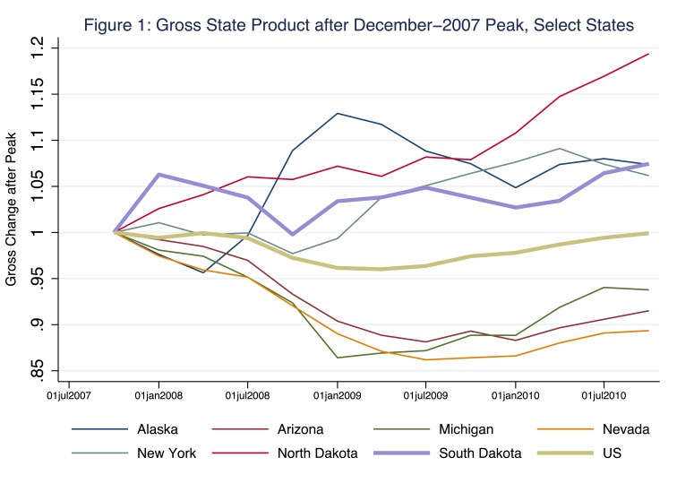
In Figure 1, we illustrate the time paths of the levels of real GSP (or, for the U.S. as a whole, GDP) relative to the level the corresponding state (or the U.S. economy) registered in December 2007—the date of the U.S. business cycle peak that preceded the Great Recession.  The y-axis value that corresponds to the fourth quarter of 2007—that is, the quarter when the economy was at its peak—is 1, the ratio of real GSP (or real GDP) at the peak to real GSP (or real GDP) at the peak; thereafter, the y-axis values correspond to either contraction—y-axis values less than one because real GSP (or real GDP) is falling relative to its value in the fourth quarter of 2007—or expansion—y-axis values greater than one because real GSP (or real GDP) is rising relative to its value in the fourth quarter of 2007.

Consider for example, the case of the U.S. (indicated in Figure 1 by the boldface, green line).  In the fourth quarter of 2007, the U.S. reached its business cycle peak, after which real GDP fell until June 2009, the business-cycle trough of the Great Recession.  Only around the third quarter of 2010 did real GDP return to the level achieved just prior to the Great Recession (and, so, around the time of the return, the boldface, green line returns to a y-axis value of 1).  The time paths for three of the states (Arizona, Michigan, and Nevada) illustrated in Figure 1 indicate GSP contractions that were deeper and longer than what the U.S. as a whole experienced.  Meanwhile, the time paths of four states, including South Dakota, illustrated in Figure 1 indicate mild, if any, GSP contractions during the Great Recession.

In Figure 2, we illustrate the unemployment rates for a selection of states and, for the sake of comparison, the United States; aside from South Dakota, we select states that, as of December 2010, registered unemployment rates that varied significantly from the U.S. unemployment rate.  In this figure, a line with a steeply positive slope indicates a rapid deterioration of the corresponding labor market.

According to Figure 2, unemployment rates generally rose as the U.S. economy entered the Great Recession.  Nevertheless, the rise was not uniform across states.  For example, while the unemployment rate in the U.S. as a whole rose to roughly two times its level before the Great Recession, the unemployment rates in Idaho and Utah nearly tripled and the unemployment rates in Alaska and North Dakota rose by roughly (and only) 25 percent of their initial levels.  As for South Dakota, initially its unemployment rate fell slightly as the U.S. economy entered the Great Recession.  Note that the y-axis indicates the gross change in unemployment, not the level of unemployment.  Thus, even though the time paths illustrated in Figure 2 for the U.S. and, say, South Dakota align quite closely, the labor market conditions during the recovery do not; put differently, by the fourth quarter of 2011, unemployment rates in both the U.S. and South Dakota nearly doubled—in the U.S., from roughly 5 to 10 percent; in South Dakota, from roughly 3 to 6 percent—though the national labor market had deteriorated more than the South Dakota labor market had.

So, recessions are not uniform across states.  And neither are expansions.

Now, consider the behaviors of aggregate economic activity and unemployment after the second quarter of 2009, the moment when the U.S. economy reached the trough of the Great Recession; at that moment, the U.S. economy began its expansion phase of the business cycle.  In Figure 3, we illustrate our measures of gross state product (GSP) for a selection of states and, again for the sake of comparison, GDP for the United States; aside from South Dakota, we select states that, by August 2019, had performed very differently than the U.S. economy as a whole.

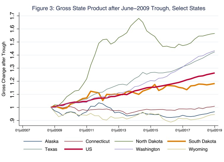
According to Figure 3, for much of the current expansion, the economies of three states (North Dakota, Texas, and Washington) outperformed the U.S. economy as a whole; meanwhile, the economies of three states (Alaska, Connecticut, and Wyoming) essentially never expanded relative to their respective 2009-trough levels!  The expansion of the South Dakota economy largely, though not entirely, mirrored the expansion of the U.S economy more generally.

In Figure 4, we illustrate unemployment rates, this time relative to their corresponding values during the business-cycle trough, for a selection of states and the United States; a steeply negative slope indicates a rapid improvement of the corresponding labor market.

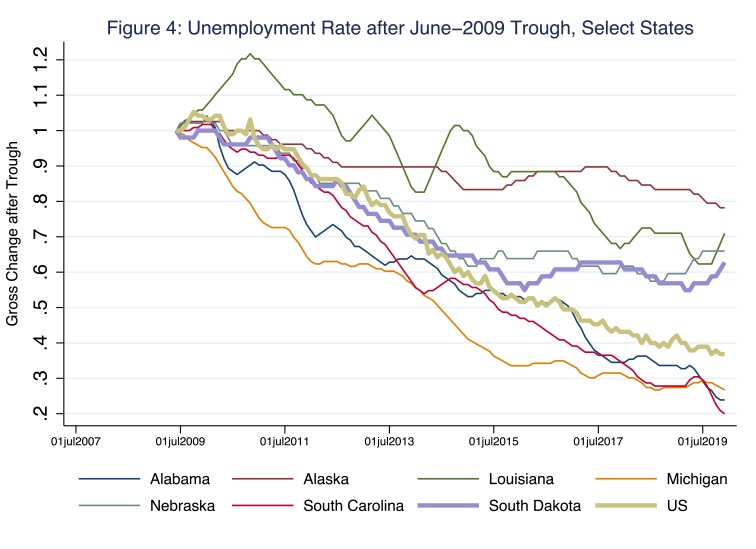
According to Figure 4, with the exception of the unemployment rate for Louisiana, unemployment rates generally fell during the expansion.  Nevertheless, the deterioration in labor markets persisted for some time in many states.  To get a sense of how the deterioration of labor markets differed over time across states, consider Figure 5, in which we somewhat unconventionally illustrate, for each state, the number of consecutive months after the June-2009 trough during which the Sahm recession indicator—or so-called Sahm rule—signaled that a recession in a particular state or the U.S. economy was imminent.

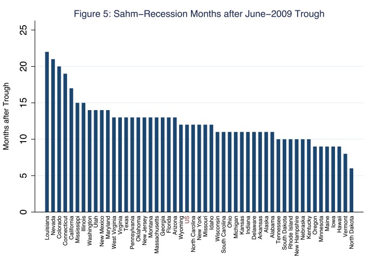
The increasingly popular Sahm Rule—named for Claudia Sahm, the director of macroeconomic policy at the Washington Center for Equitable Growth and formerly with the Board of Governors of the Federal Reserve—signals a macroeconomic recession (though here we take the liberty of applying it to individual states) when the three-month-average unemployment rate rises by at least a half of a percentage point above the lowest three-month-average monthly unemployment rate in the previous 12 months.  (And, yes, the Sahm rule is a pretty good indicator of impending macroeconomic recession.)  According to Figure 5, the Sahm rule continued to signal recession in the US (x-axis label in red font near the middle of Figure 5) for twelve consecutive months after June 2009.  For the states indicated to the left [right] of the U.S. in Figure 5, the Sahm rule continued to signal recession in those states for more [less] than 12 months.  So, for example, in the case of Louisiana (far left of Figure 5), the Sahm rule continued to signal recession for 22 consecutive months—nearly two years!—after the June-2009 business-cycle trough.

Not surprisingly, perhaps, because the effects of business cycles tend to vary across states, state-level variation in unemployment rates tends to increase during contractions, when the cyclical strains on labor markets across the country are not uniform.  This pattern is apparent in Figure 6, in which we illustrate a times series plot of simple monthly standard deviations—think, average variation in percentage-point terms—of state-level unemployment rates; we include gray bars to indicate U.S. contractions determined by the National Bureau of Economic Research (NBER).

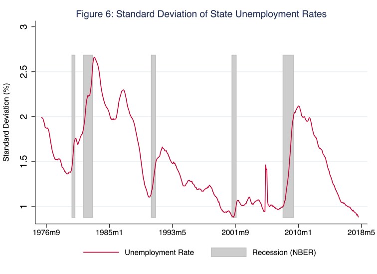
So, for example, according to Figure 6, during the Great Recession, the monthly standard deviation of state-level unemployment rates reached about 2.2 percent.  During expansions, which are typically longer than contractions, unemployment rates fall and, over time, converge across states thanks, in part, to interstate labor mobility.  Thus, outside the ranges of the gray bars in Figure 6, the monthly standard deviations of state-level unemployment rates tend to fall.  Finally, although in this blog post we mostly focus on the Great Recession, the patterns of state-level heterogeneity that we demonstrate here are apparent in business cycles more generally; indeed, this generality is apparent in Figure 6, which includes data back to 1975 and, thus, five macroeconomic contractions.

U.S. fiscal and monetary policy responses to the economic crisis spurred by the novel coronavirus are rightly large, and unprecedentedly so.  And we are not done.  The economic losses imposed by the novel coronavirus will be on an order of magnitude of the economic losses imposed by the Great Recession.  The macroeconomic policies we implement to tackle the crisis must address heterogenous state-level economic performance: each of the fifty states experience business cycles—the downturns and the recoveries—differently, sometimes dramatically so.  One-size-fits-all stabilization policies are not ideal.  A customized approach is necessary; fiscal policy is relatively well suited to the task.