This blog post accompanies the SDPR Morning Macro segment that aired Monday, March 4.

Last week, the Bureau of Economic Analysis, a unit of the U.S. Department of Commerce, reported that real gross domestic product (GDP) grew in the fourth quarter of 2018 by an annualized rate of 2.6 percent, less than the annualized rate of 3.4 percent that real GDP grew in the third quarter of 2018.  Economists (and everyone else) waited anxiously for the report, which they parsed and analyzed in excruciating detail—just as they had every quarter before.

Last spring, the Economist magazine criticized the economics profession for relying on erroneous measures of what it called the worth of nations—GDP and its components, for the most part.  Though this critique is not new, the implications for how we measure, analyze, and influence (with policy) the macroeconomy remain profound.  The macroeconomy refers to the economy as a whole, its general features.  These features pertain primarily to aggregate production, the purchasing power of money, and its time value—GDP and its components, for the most part.  I’ll return to the critique in a moment; but first, what is GDP?

GDP measures the market value of all final goods and services produced within an economy over an interval of time, typically over a year.  In the United States, the BEA computes and reports on GDP each quarter.  The BEA gathers the necessary information from many data sources, including, for example, tax documents.  Generally speaking, we can think about GDP two ways: namely, the total income of everyone participating in the economy, or the total expenditure—by households, firms, governments, and foreigners—on the economy’s output of goods and services.  Both ways of thinking about GDP are valid, because for the economy as a whole, domestic income must equal domestic expenditure; or, put differently, every transaction has a seller—think, income—and a buyer—think, expenditure.

Because GDP measures the market value of goods and services produced, GDP changes over time as market values change—that is, as the prices of goods and services produced change—and as the quantities of goods and services produced change.  Thus, essentially, over time two broad forces move GDP: namely, prices and quantities.  Incidentally, we refer to this measure of GDP—which values produced quantities at current prices—as either nominal GDP or, simply, GDP.  In Figure 1, I illustrate a time series of U.S. GDP from 1960 to the present.

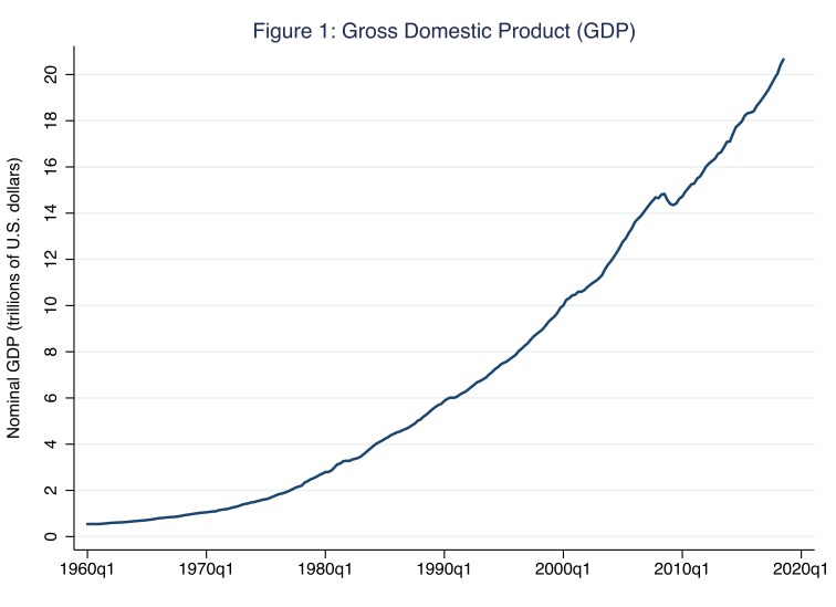
In 1960, U.S. GDP measured roughly $0.5 trillion; whereas in 2018, U.S. GDP measured roughly $20.7 trillion.  Thus, between 1960 and 2018, GDP grew on (geometrical) average roughly 6.5 percent annually.  A portion of this 6.5 percent annual growth was due to increases in prices—that is, due to inflation, the subject of a future Morning Macro segment—and a portion of this annual growth was due to increases in produced quantities of goods and services.  Moreover, the annual growth of GDP from 1960 to 2018 was not steady; for example, in Figure 1 we can easily identify the combined effects on prices and quantities of the recession around 2008.

In any case, if economists wish to study the macroeconomic effects of changes in produced quantities only, we look to real GDP, which measures the market value, based on prices in a so-called base year, of all final goods and services produced.  Put differently, in order to compute real GDP, the BEA effectively purges nominal GDP of the effects of inflation.  In Figure 2, I illustrate a time series of real GDP alongside nominal GDP, both over the sample period of 1960 to the present; in this case, real GDP values produced quantities at prices in base-year 2012, when nominal and real GDP are necessarily identical and, thus, where the lines cross in Figure 2.

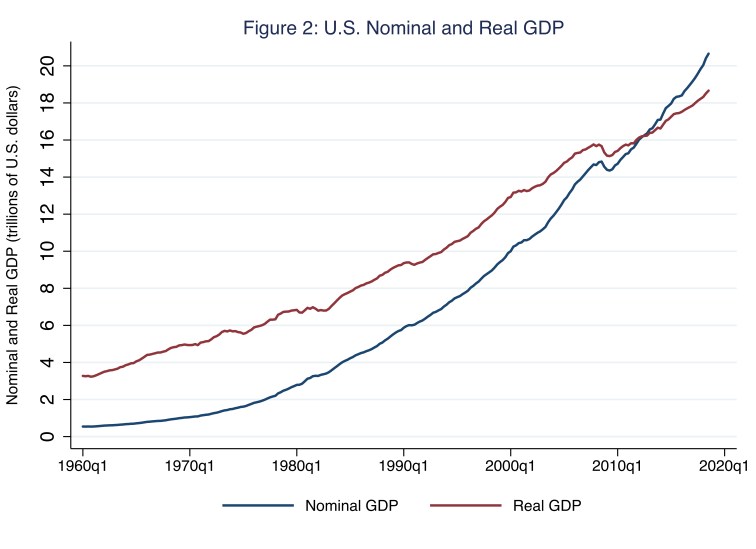
Notice, our interpretation of real GDP is entirely specific to changes in produced quantities as opposed to changes in prices: in 1960, U.S. real GDP measured roughly $3.2 trillion in 2012 prices; whereas in 2018, U.S. GDP measured roughly $18.7 trillion in 2012 prices.  Thus, between 1960 and 2018, real GDP grew on (geometrical) average roughly 3.1 percent annually.  This is to say, because real-GDP market values, measured by base-year 2012 prices, do not change over time, we know this 3.1 percent annual growth is due entirely to increases in produced quantities of goods and services.  As with nominal GDP, the annual growth of real GDP from 1960 to 2018 was not steady; though, because real GDP is not influenced by the effects of inflation, in Figure 2 we can easily identify the effects on output of several recessions: for example, those around 1974, 1980, 1981, 1990, 2001, and, of course, 2008.  Incidentally, because the U.S. experienced a general rise in prices from 1960 to the present, real GDP is necessarily greater [less] than nominal GDP before [after] base year 2012.

Nominal and real GDP are extremely useful measures of macroeconomic activity.  For example, real GDP allows us to quantify and, thus, study (long-run) economic growth and (short-run) business cycles—irregular expansions and contractions in economic activity over time in the economy as a whole.  And, to be sure, the BEA’s work computing GDP and other measures pertaining to the national income and product accounts more generally is little short of amazing.  Nevertheless, GDP is an imperfect economic statistic, particularly when we use it to measure well-being, or what economists refer to as standards of living.  This imperfection is the gist of the Economist magazine’s critique to which I refer in my opening paragraph.

Our profession’s conventional measure of standard of living is real GDP per capita over time, which I illustrate in Figure 3 for the United States.

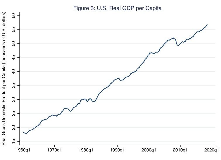
By this measure, in 1960, the U.S. standard of living measured roughly $18 thousand per person (in 2012 prices); whereas in 2018, the U.S. standard of living measured roughly $57 thousand per person (in 2012 prices).  Thus, between 1960 and 2018, the U.S. standard of living grew on (geometrical) average roughly 2 percent annually.  Put differently, then, on average, the U.S. standard of living has doubled about every 35 years since 1960.

Drawing such conclusions is problematic, of course.  First, real GDP per capita is, at best, an average level of aggregate income that, by definition of an average, no individual in the economy necessarily earns.  As Glenn Hubbard, dean of Columbia Business School, noted last year in a  Wall Street Journal interview, average [income per capita] is not always entirely useful.  Hubbard reasons that economists would do well instead to consider human dignity.  Second, GDP measures market transactions; thus, by definition, GDP omits positive externalities from, say, education and negative externalities from, say, air pollution.  GDP also misses non-market activities such as work at home, leisure, and illicit transactions.  And third, the value of GDP is measured in units of money, which has diminishing marginal value: the more income one has, the less she values (and the more willing she is to surrender) an additional unit of income measured, of course, in units of money.

Indeed, Roberto Stefan Foa and Yascha Mounk, in an essay published just days ago in the Wall Street Journal, incidentally showcase the moral indifference of GDP when they acknowledge the alarming likelihood that within the next five years or so, “The combined economies [measured by GDP] of democratic countries like the U.S., Germany, France and Japan will be smaller than those of autocracies like China, Russia, Turkey and Saudi Arabia.”  Clearly, GDP tells us nothing about the extent to which an economy’s participants experience the personal and political freedoms we hold so dear.

In the last few decades, economists have proposed many alternative measures of the standard of living, including the often-cited United Nations Human Development Index.  (For some context, see this short Project Syndicate In Theory piece.)  Consider the equivalent-income approach of Fleurbaey and Gaulier (2007), who adjust GDP per capita for non-market-income features of life and the distribution of income in twenty-four countries listed in Table 1 (which appears as Figure 2 on page 24 of their paper).

Table 1: GDP per capita and Its Adjustment for Living Standards, 2004 PPP US$

	GDP per cap and ranking		Adjustment and ranking
Austrailia	$      30,116	13	$      26,508	19
Austria	$      32,176	7	$      34,695	5
Belgium	$      31,009	11	$      28,366	15
Canada	$      31,129	10	$      28,414	14
Denmark	$      31,974	9	$      29,689	12
Finland	$      29,816	14	$      26,034	20
France	$      29,077	17	$      32,805	8
Germany	$      28,147	19	$      27,276	18
Greece	$      21,954	22	$      22,582	21
Iceland	$      33,090	6	$      31,972	9
Ireland	$      40,058	2	$      39,782	3
Italy	$      28,162	18	$      30,442	11
Japan	$      29,539	15	$      34,989	4
Korea	$      20,371	23	$      21,653	22
Luxembourg	$      68,719	1	$      55,828	1
Netherlands	$      32,056	8	$      31,348	10
New Zealand	$      22,912	21	$      21,320	23
Norway	$      38,288	4	$      39,975	2
Portugal	$      19,687	24	$      19,163	24
Spain	$      25,341	20	$      28,131	16
Sweden	$      29,499	16	$      28,027	17
Switzerland	$      33,541	5	$      33,701	6
U.K.	$      30,843	12	$      29,233	13
U.S.	$      39,618	3	$      33,315	7

The authors’ results imply that, for some countries, GDP per capita grossly misses the mark as a measure of the standard of living.  For example, the United States falls four places in the ranking (from third place based solely on GDP per capita to seventh place based on the adjusted measure), Australia and Finland fall six places, and Japan rises eleven places.

These and other such measurement errors should inform how we set macroeconomic policy objectives against which we evaluate—and, thus, measure—policy outcomes.  Despite our best intentions, our imprecise descriptions and measures of the human condition conveyed by terms such as standard of living, employment, poverty, or inflation compromise the effectiveness of our macroeconomic policy.  In macroeconomic policy, as in social interventions more generally, we often get what we measure; so we should measure carefully.

For more information on the principal concepts of macroeconomic policy, including the challenges of evaluating policy on the basis of empirical measures of macroeconomic outcomes, see Chapter 1 of the second edition of Bénassy-Quéré, Agnès, Benoît Cœuré, Pierre Jacquet, and Jean Pisani-Ferry, Economic Policy: Theory and Practice (Oxford: Oxford University Press, 2018).

Additional References

Fleurbaey, Marc and Guillaume Gaulier.  2007.  “International Comparisons of Living Standards by Equivalent Incomes.”  CEPII working paper 2007–03, January.