This blog post accompanies the SDPR Morning Macro segment that aired Monday, February 25.

In February 2014, the White House Council of Economic Advisors reported the American Recovery and Reinvestment Act of 2009, which Congress passed in response to the Great Recession, had generated annually 1.6 million jobs and 2 to 3 percentage points of gross domestic product from 2009 to 2011.  More recently, in a July 2018 post on Whitehouse.gov, Secretary of the United States Treasury, Steven T. Mnuchin, attributed the U.S. economy’s ongoing job and income growth to the Tax Cuts and Jobs Act of 2017, which President Trump signed into law on December 22, 2017.

Such claims (by members of either political party) regarding how the economy is shaped by fiscal policy—that is, discretionary government spending or taxing intended to change cyclical features of the macroeconomy, such as relatively high unemployment—intrigue macroeconomists.  This is because identifying empirically how the economy responds to fiscal policy is very difficult work.  Although we observe changes in government spending or taxing along with, say, changes in output, how do we know such government interventions cause changes in output?

Essentially, the problem is that our fiscal-policy measure—changes in government spending or taxing—may reflect existing or anticipated features of the economy; that is, the measure may be endogenous.  For example, suppose changes in government spending reflect existing features of the economy because the measure is pro-cyclical.  In this case, the effect of government spending on output seems stronger than it actually is, because spending and output both rise [fall] as the economy expands [contracts].  Alternatively, suppose changes in taxes reflect anticipated features of the economy because the policy maker cuts taxes when she (correctly) anticipates a recession.  In this case, the effect of a tax cut on output seems weaker than it actually is, because output falls as the economy contracts.  Thus, the solution is to find an exogenous fiscal-policy measure—one that does not reflect existing or anticipated features of the economy.

Spoiler alert: economists disagree on what constitutes an exogenous measure.

Empirical evidence of the macroeconomic effects of fiscal policy is mixed, at best.  The research on this subject is extensive; and, perhaps not surprisingly, much of it is loosely inspired by, though rarely modeled around, the highly stylized, Keynesian framework of government spending and taxing multipliers—the sort we all studied in principles of macroeconomics class.  For example, increases in government spending increase output, consumption, and employment; increases in taxes do the opposite.  Often, an implicit assumption of this oversimplified framework is that fiscal policy, which intends to move economic activity to the level associated with full employment, improves welfare: stabilization policies make us better off.  To gain a sense of the research on this topic, consider two renowned studies, one of spending and the other of taxing.

Valerie A. Ramey and Matthew Shapiro (1998) regress output, consumption, and other macroeconomic variables on a fiscal-policy measure they construct from government spending on military buildups in the United States between 1947 and 1996.  According to the authors, “because they are driven by geo-political shocks, military buildups are likely to be exogenous with respect to macroeconomic variables” (Ramey and Shapiro, 1998, p. 174).  Based on narrative records, including articles in Business Week magazine, the authors date buildups to 1950 (the Korean War), 1965 (the Vietnam War), and 1980 (the Carter-Reagan buildup).  The authors find government spending increases defense-related output while it ultimately decreases private output and consumption.  These results are broadly consistent with a neoclassical—not Keynesian—framework.

Christina D. and David H. Romer (2010) regress output on a fiscal-policy measure they construct from legislative tax changes passed in the United States between 1945 and 2007.  Based on narrative records (published, for example, in various issues of the Economic Report of the President and the Congressional Record), the authors identify so-called exogenous tax changes, which they define as “those not taken to offset factors pushing [output] growth away from normal” (Romer and Romer 2010, 770).  As a practical matter, the authors find that exogenous tax changes are usually taken to pay down existing debt or increase long-run growth.  The authors find tax increases are highly contractionary.  Thus, according to their work, tax increases affect output and consumption in ways that are at least broadly consistent with a Keynesian framework.

Though empirical evidence of the macroeconomic effects of fiscal policy are mixed, the immediate budgetary consequences of fiscal policy are clear: changes in government spending and taxing change the budgetary position of the federal government and, in turn, its debt position.  Understanding how fiscal policy shapes long-term government budgets and debt is important.  The federal budget is a plan that identifies intended government receipts—tax revenues and social-insurance contributions, for example—and expenditures over a specified time period, typically a fiscal year.  The budget balance is the difference between receipts and expenditures; economists refer to negative and positive balances as deficits and surpluses, respectively.  In Figure 1, I illustrate the U.S. federal budget balance, as a percentage of GDP, since 1970.

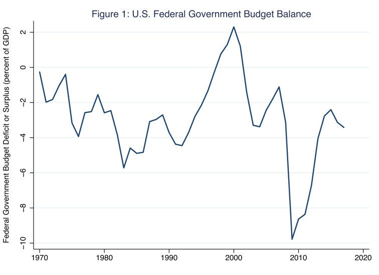
Between 1970 and 2017, the U.S. government maintained a budget surplus from 1998 to 2001, only.  The enormous increase in the budget deficit that began in 2009 was driven by a slowing economy (and, thus, lower tax revenues and higher automatically stabilizing expenditures) and the American Recovery and Reinvestment Act.  Figure 1 does not reflect the 2017 tax reform (known as the “Tax Cuts and Jobs Act”) that Congress passed and President Trump signed into law in December 2017.  According to the nonpartisan Congressional Budget Office (CBO), all else equal, this tax reform will increase the deficit (in absolute value) by $1.5 trillion over the next 10 years.  The reform will increase the budget deficit, as a percentage of GDP, from 3.4 percent (in fiscal year 2017) to 5.1 percent (in fiscal year 2028).

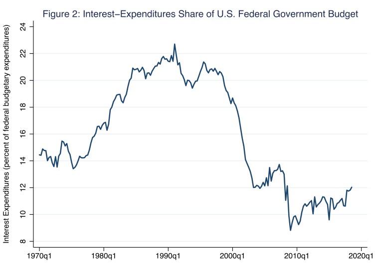
The budget balance (as a percentage of GDP) that I illustrate in Figure 1 is, formally speaking, the total fiscal balance, which we also refer to as the financial balance.  It is the difference between receipts and expenditures, including interest expenditures paid on the public debt—over $550 billion in 2018, or, as Figure 2 illustrates, about 12 percent of all federal government expenditures that year.

The debt is the negative net accumulation of financial deficits and surpluses.  The financial balance represents the total borrowing needs of the federal government in a given fiscal year.  Of course, in a given fiscal year, interest expenditures are predetermined by the level of debt and borrowing rates of interest; put differently, interest expenditures are not determined by current budgetary actions.  Thus, a more-suitable measure of current budgetary actions is the primary balance, defined as the financial balance excluding interest expenditures paid on the public debt as follows.

Financial balance = primary balance – interest payments

For example, if the primary balance is -$100 and interest payments are $50, the financial balance is -$150.  In this example, the financial balance of -$150 is comprised of two parts: a negative balance of $100 determined by current budgetary actions minus expenditures of $50 predetermined by the levels of debt and borrowing rates of interest.

So, essentially, the debt drives the difference between financial and primary balances, because the size of the debt determines the size of interest payments on the debt.  As the debt increases and, thus, interest payments increase, the debt burden—think, budget constraint—on current budgetary actions increases as well.  In Figure 3, I illustrate the U.S. federal (public) debt, as a percentage of GDP, since 1970.

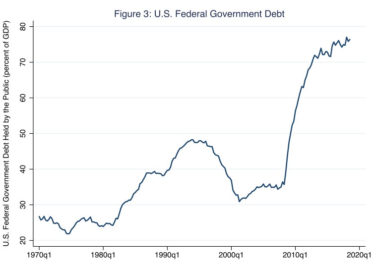
Between 1970 and 2017, the U.S. federal debt, as a percentage of GDP, rose from 27 percent in 1970 to 75 percent in 2017.  The enormous increase in the debt that began in 2009 was driven arithmetically by the enormous increase in the deficit at that time (Figure 1).  This is because deficits are negative budgetary flows that accumulate into debt.  Like Figure 1, Figure 3 does not reflect the 2017 Tax Cuts and Jobs Act.  According to the CBO, all else equal, this tax reform will increase the debt, as a percentage of GDP, from 75 percent (in fiscal year 2017) to 89 percent (in fiscal year 2028).  This debt-to-GDP ratio attracts lots of attention, particularly now, when it is about 75 percent.  How much debt is too much?  One way to approach this question is from the perspective of sustainability: assess whether the debt-to-GDP ratio is in a (constant) steady state.

To do so, consider the dynamic process that determines the debt (at time t); this process is described by the following expression.

B_t = (1 + i)B_t-1 + D_t

Where B and D are, respectively, the debt and the primary deficit; i is the nominal interest rate, which we define as the real interest rate plus the expected inflation rate.  The current period’s debt (B_t) is the sum of three parts: the prior period’s debt (B_t-1), the interest payment on the prior period’s debt (i×B_t-1), and the current period’s primary deficit (D_t).  (Incidentally, the financial deficit is, i×B_t-1 + D_t.)  Dividing both sides of the prior expression by nominal GDP at time t yields the following approximation.

b_t ≈ (1 + i – n)b_t-1 + d_t

Where b and d are, respectively, the debt and primary deficit as percentages of (contemporaneous) nominal GDP; n is the growth rate of nominal GDP.  If the debt-to-GDP ratio (b) is in a steady state, then b_t = b_t-1.  Imposing this steady-state condition on the prior expression (and dispensing with time subscripts) yields the following steady-state relationship between the deficit and the debt, as percentages of GDP, the nominal interest rate, and GDP growth rate.

d + ib ≈ nb

The left side of this expression is the financial deficit; the right side is the amount the debt must grow so that the debt-to-GDP ratio remains constant.  (Recall, n is the growth rate of GDP.)  In plain English, in order for the debt-to-GDP ratio to remain constant, the financial deficit must grow the debt by no more than the growth rate of GDP.

So, with this steady-state relationship is mind, is the U.S. federal debt-to-GDP ratio sustainable?  Consider Table 1, in which I report the results of a simple simulation exercise based on the prior steady-state expression.  In this table, I assume the growth rate of nominal GDP is 5 percent; that is, n = .05.  For each of five nominal-interest rate scenarios (in rows 1 through 5), I report in column two the steady-state deficit-to-GDP ratio required to maintain the 2017 U.S. debt-to-GDP ratio of 75 percent.  In column three I report the actual 2017 U.S. deficit-to-GDP ratio.

Table 1: Debt-to-GDP Stabilization Exercise based on U.S. Data for 2017

Nominal Interest Rate	Steady-State Deficit	Actual Deficit
1.0%	3.0%	3.4%
2.0%	2.3%	3.4%
3.0%	1.5%	3.4%
4.0%	0.8%	3.4%
5.0%	0.0%	3.4%

For example, consider row two, where the interest rate is 2 percent.  In this case, for the U.S. debt-to-GDP ratio to remain at 75 percent (or less), the deficit-to-GDP ratio must remain at 2.3 percent (or less).  Because the actual deficit-to-GDP ratio is 3.4 percent, the debt-to-GDP ratio is not in a (stable) steady state; rather, it is rising.  The steady-state deficit decreases—and, thus, the fiscal budget constraint tightens—as the interest rate rises.  Perhaps most importantly, the constraint also tightens as the growth rate of GDP falls.  For example, suppose an interest rate of 5 percent and a growth rate of GDP of 3 percent.  In this case (which Table 1 does not report), for the U.S. debt-to-GDP ratio to remain at 75 percent (or less), the surplus-to-GDP ratio must be 1.5 percent (or more).  No wonder the CBO estimates the recent tax reform will increase the debt-to-GDP ratio.

Additional References

Alberto Alesina and Francesco Giavazzi (ed.)  2013.  Fiscal Policy after the Financial Crisis.  Chicago, IL: University of Chicago Press.

Ramey, Valerie A. and Matthew D. Shapiro.  1998.  “Costly capital reallocation and the effects of government spending.” Carnegie-Rochseter Conference Series on Public Policy, 48, 145-194.

Romer, Christina D. and David H. Romer.  2010.  “The macroeconomic effects of tax changes: Estimates based on a new measure of fiscal shocks.”  American Economic Review, 100, 763-801.