This blog post accompanies the SDPR Morning Macro segment that airs on Monday, April 29.

In The General Theory of Employment, Interest, and Money, John Maynard Keynes (1936) observed,

“Practical men, who believe themselves to be quite exempt from any intellectual influences, are usually slaves of some defunct economist.  Madmen in authority, who hear voices in the air, are distilling their frenzy from some academic scribbler of a few years back” (383).

In 1958, Alban William (A. W.) Phillips, then a professor at the London School of Economics, published, “The Relation between Unemployment and the Rate of Change of Money Wage Rates in the United Kingdom, 1861-1957.”  In it, Phillips analyzed “whether statistical evidence supports the hypothesis that the rate of change of money wages in the United Kingdom can be explained by the level of unemployment…” (Phillips 1958, p. 284).  (Today, we typically refer to the money wage—the wage measured in dollars, say—as the nominal wage or, simply, the wage; though any one of these terms is acceptable.)  Controlling for large increases in import prices, Phillips concluded statistical evidence supported the hypothesis: relatively low [high] unemployment rates drive relatively high [low] rates of change of money wages.  To illustrate this, Phillips (1958) included several scatter diagrams, including the following, which he labeled Fig.1.

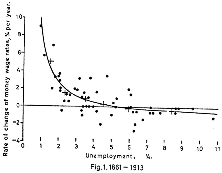
Each point in the illustration represents the unemployment rate (read off the x-axis) and the rate of change of the wage (read off the y-axis) for a particular year from 1861 through 1913.  The smoothed, fitted line in the figure captures the essential takeaway of Phillips’s statistical analysis.  We can think of this line as the original Phillips curve—generally speaking, a trade-off between the unemployment rate and the inflation rate (captured here as the rate of change of the wage, which is highly positively correlated with the inflation rate).  The idea of this trade-off has had enormous intellectual influence in macroeconomic theory—think, new-Keynesian Phillips curve—and policy—think, Federal Reserve dual mandate of high employment and low and stable inflation.  Without exaggeration, we could say the Phillips curve revolutionized macroeconomic policy.  Yes, in the pantheon of macroeconomists, A. W. Phillips is a leading “academic scribbler, ” second only, perhaps, to J. M. Keynes.

The Phillips-curve trade-off almost immediately gained international acclaim.  For roughly a decade after Phillips (1958) published his analysis of the U.K. economy, the U.S. economy seemed to demonstrate a similarly reliable trade-off.  For example, consider Figure 1, in which I plot for the United States a scatter diagram of the annual unemployment rate and the annual growth rate of average hourly wages (measured here as earnings, in dollars, of production and nonsupervisory employees in manufacturing) for each of the years 1960 through 1969.  The red line is a fitted linear trend that I include, much as Phillips (1958) did in his illustration above, as a visual aid to emphasize the pattern of a trade-off: throughout the decade of the 1960s, relatively low [high] unemployment rates were associated with relatively high [low] wage-growth rates.

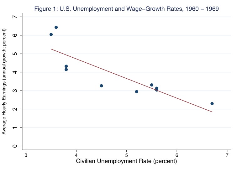
Near the start of the decade, in 1961, the U.S. unemployment rate averaged 6.7 percent while the wage-growth rate averaged 2.3 percent; the point representing these coordinates is nearest to the lower, right-side corner of the figure.  Eight years later, in 1969, the unemployment rate averaged 3.5 percent while the wage-growth rate averaged 6.0 percent; the point representing these coordinates is nearest to the upper, left-side corner of the figure.  Moreover, the rather precisely fitted trend illustrates that, in most of the intervening years, unemployment rates and wage-growth rates (and, more generally, inflation rates) moved in opposite directions.

In the 1960s—the heyday of Keynesian macroeconomic stabilization policy—many economists read the Phillips curve as a so-called policy menu of macroeconomic outcomes from which the policymaker could simply choose by managing aggregate demand accordingly.  For example, according to Figure 1, if the policymaker wished for 5.5 percent unemployment, she could stimulate wage growth of about 3 percent, by stimulating aggregate demand—think, total expenditures by consumers and firms—and, thus, inflation through monetary or fiscal policy, say.  Indeed, in his conclusion, Phillips (1958) alluded to just such a menu-driven stabilization-policy approach when, referring to his Fig.1 that I illustrate above and using the examples of 2.5 percent and 5.5 percent unemployment rates, he wrote,

“…it seems from the relation fitted to the data that if aggregate demand were kept at a value which would maintain a stable level of product prices the associated level of unemployment would be a little under 2½ per cent.  If, as is sometimes recommended, demand were kept at a value which would maintain stable wage rates, the associated level of unemployment would be about 5½ per cent” (299).

Nevertheless, a policy menu of these macroeconomic outcomes—one real (the unemployment rate) and one nominal (the inflation rate)—struck some economists as unworkable, particularly in the long run.  This is because real labor-market forces, reflected in, say, the rates of job search and separation, determine the natural rate of unemployment (Friedman 1968; Phelps 1968).  (For more on the natural rate of unemployment, see the Morning Macro segment, “Separation Anxiety.”)  Meanwhile, nominal macroeconomic-policy-induced forces, such as increases in the money stock, determine the price level and, thus, the nominal wage, its growth rate, and the inflation rate more generally.  According to this classical (real-nominal) dichotomy, the trade-off between the unemployment rate and the inflation rate is not permanent; indeed, the trade-off is, for all practical purposes, nonexistent.  If anything, it lasts only until prices and wages adjust to the policy-induced inflation; and the time length of this adjustment is determined by how individuals—employees and employers, for example, who negotiate wages with inflation rates in mind—formulate expectations of inflation.

Revolution was in the air.

In principle, if individuals rightly expect, say, a rise in the inflation rate, they preemptively  adjust prevailing prices and wages in order to preserve their market-clearing levels in real terms—that is, in terms of the goods and services whose values these prices and wages measure.  Consequently, the rise in the inflation rate does not affect the economy’s real features, including the real wage, the level of employment, and the unemployment rate; thus, Phillips-curve trade-offs are fleeting events that policymakers cannot exploit.  This means macroeconomic stabilization policies affect real features of the economy only if individuals systematically fail to expect changes in the inflation rate.  Such systematic failures occur because individuals neglect to learn from their mistakes, even though such neglect is costly.  Why would individuals neglect to minimize cost in this way?  According to the rational-expectations hypothesis, they would not.

Rather, according to the rational-expectations hypothesis, individuals formulate expectations of  the inflation rate (and all else) using all available information; moreover, individuals interpret this information based on an accurate understanding of their complex economic environment.  Thus, rational expectations are determined within the economic model that determines the inflation rate and all other such variables.  (For a detailed technical exposition on how individuals formulate rational expectations, see the Appendix below.)  Put differently, then, in the context of Figure 1, Phillips curves are vertical in the long run: as the labor market tightens, and wage-growth and inflation rates rise, the unemployment rate remains near its full-employment level; the unemployment rate does not fall persistently below its natural rate.

The rational-expectations hypothesis instigated a revolution in macroeconomics that changed how we thought about macroeconomic policy.  Meanwhile, circumstances transpiring in the real economy fueled the revolution; as in life, in macroeconomics timing is everything.  The rational-expectations revolution in the 1970s seemed to usher in a vertical Phillips curve.  In Figure 2,  I plot a scatter diagram of the annual unemployment rate and the annual growth rate of average hourly wages (measured here as earnings, in dollars, of production and nonsupervisory employees in the private sector) for each of the years 1970 through 1979.

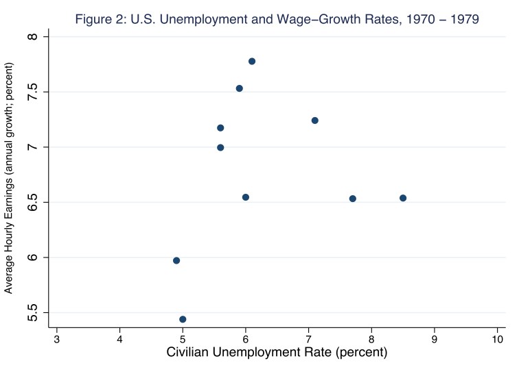
A downward-sloping Phillips curve is absent from Figure 2.  Rather, the unemployment rate seems largely independent of wage growth, much as the rational-expectations hypothesis predicts.  For example, while wage growth during the decade varies from between about 5 to 8 percent, the unemployment rate mostly hovers around 6 percent.  The rational-expectations revolution seemed to settle the debate: the unemployment rate cannot remain below its natural rate for long without fueling relatively high wage growth and inflation more generally.

Yeah, about that…

Since the Great Recession, the unemployment rate has fallen from a peak of 10 percent reached in October 2009 to 3.8 percent today.  According to the Congressional Budget Office, which estimates the natural rate of unemployment, the current unemployment rate is about 0.8 percent below the natural rate, a relationship that presumably signals a relatively tight labor market—one in which wage growth and inflation more generally should rise.  Instead, since the Great Recession, wage growth and inflation have not risen substantially.  In Figure 3, I plot a scatter diagram of the annual unemployment rate and the annual growth rate of average hourly wages for each of the years 2009 through 2018, when the Phillips curve is anything but vertical: in fact, it is essentially horizontal.

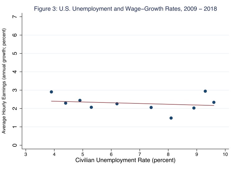
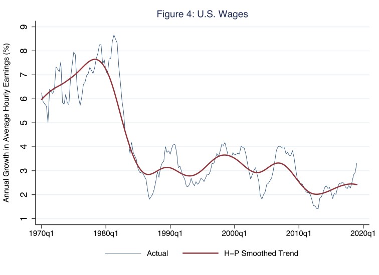
In 2010, shortly after the U.S. economy exited the business-cycle trough of the Great Recession, the unemployment rate averaged 9.6 percent while the wage-growth rate averaged 2.3 percent; the point representing these coordinates is nearest to the right side of the figure.  Eight years later, in 2018, the unemployment rate averaged 3.9 percent while the wage-growth rate averaged 2.9 percent; the point representing these coordinates is nearest to the left side of the figure.  Moreover, the rather precisely fitted trend illustrates that, in most of the intervening years, the wage-growth rate (and, more generally, the inflation rate) was largely independent of the unemployment rate.  The relatively weak wage growth since the Great Recession is apparent in Figure 4, in which I include a non-linear smoothed trend in order to capture the general decline in wage growth since the 1970s and, more recently, since the Great Recession.  Only in the last few years has wage growth picked up—in the U.S. and, incidentally, in Phillips’s U.K.

So why has wage growth remained around 2.5 percent while the labor market has tightened and the unemployment rate has fallen below its natural rate?  Generally speaking, two principal forces drive wage growth: inflation—think, the rate of decline in the purchasing power of money—and labor-productivity growth—think, the rate of growth of output per hour of labor input.  In theory, if the labor market clears—labor supply equals labor demand—and neither employers nor employees have market power (to manipulate wages, for example), then the following relationship holds.

Wage Growth Rate = Inflation Rate + Labor-Productivity Growth Rate

Incidentally, we can think of a Phillips curve as the relationship between the unemployment rate and the wage-growth rate holding the labor-productivity growth rate constant.  In Figures 5 and 6, I plot, respectively, the inflation rate and the labor-productivity growth rate; for the latter, I include a non-linear smoothed trend as a visual aid.

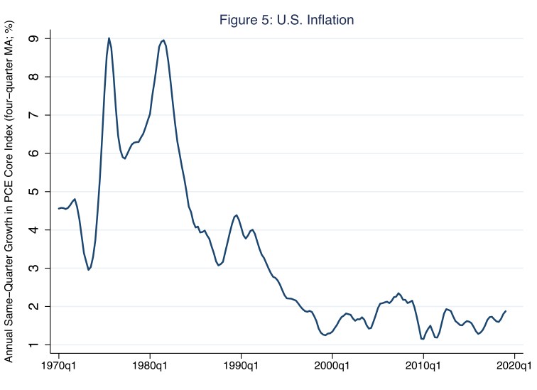
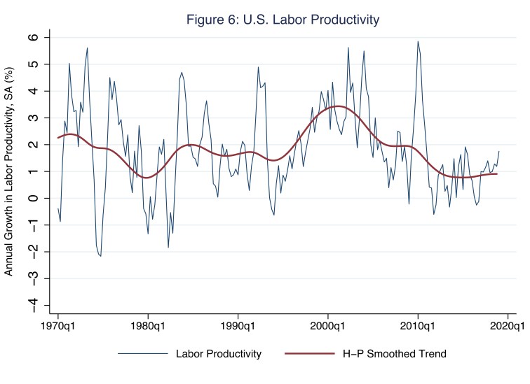
According to Figures 5 and 6, since at least the Great Recession, the two principal forces driving wage growth have reached historically low levels.  The inflation rate, measured in Figure 5 as the growth in the core personal consumption expenditures index, has hovered below the Fed’s target level of 2 percent.  Meanwhile, labor-productivity growth has hovered just below 1 percent.  In Table 1, I report, for several decades, the growth rates of hourly compensation—a broad measure of the nominal wage—and its principal drivers: inflation and labor-productivity growth.  For each decade listed, annual growth in hourly compensation—think, wage growth rate—is roughly equal to the inflation rate plus the labor-productivity growth rate, just as economic theory predicts.  Notice, the growth rates reported in the last row of Table 1 are exceptionally low.

Table 1: Growth in U.S. Hourly Compensation and Its Principal Sources

	Compensation (%)	Inflation (%)	Productivity (%)
1950 – 1959	5.3	2.5	2.6
1960 – 1969	4.8	2.4	2.7
1970 – 1979	8.0	6.5	2.0
1980 – 1989	5.6	4.4	1.5
1990 – 1999	3.9	2.1	2.2
2000 – 2009	3.6	2.2	2.7
2010 – 2018	2.3	1.7	0.9

Frankly, why recent inflation rates and labor-productivity growth rates have been so relatively weak are two puzzles that macroeconomists have yet to solve.  The inflation puzzle regards the Phillips curve—specifically, why is the curve horizontal while the unemployment rate is persistently below its natural rate?  Nevertheless, of these two puzzles, macroeconomists agree that weak labor-productivity growth is the greatest threat to economic well-being.  This is because labor-productivity growth essentially determines the growth of real hourly compensation—the growth in the purchasing power of (nominal) wages.  Not surprisingly, wage earners care most about real hourly compensation.  In Figure 7, I plot the growth of real hourly compensation, which, on trend, has hovered below 1 percent since the mid 2000s, at least three years before the Great Recession.

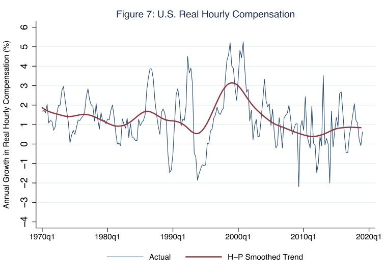
Finally, in Figure 8, I combine the smoothed trend in the growth of real hourly compensation (Figure 7) and the smoothed trend in the growth of labor productivity (Figure 6).  As economic theory predicts, the two smoothed series roughly align.

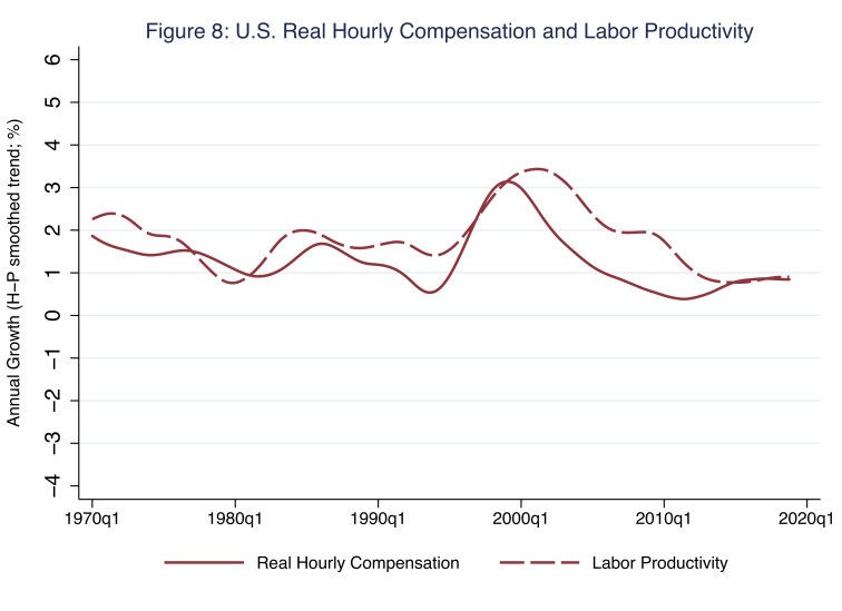
According to Figure 8, from the early 2000s until about 2015, the growth of real hourly compensation lagged the growth of labor productivity—the dashed line is above the solid line in Figure 8.  Put differently, from the early 2000s until about 2015, nominal wages did not keep pace with inflation.  In any case, as the labor market has tightened in the last few years, the growth of real hourly compensation has converged on the growth of labor productivity—after 2015, the two lines in Figure 8 essentially overlap.  On the one hand, this is good news for labor, because nominal wages are finally keeping pace with inflation, and so real hourly compensation is finally keeping pace with labor productivity.  On the other hand, this is bad news, because the growth of labor productivity remains historically low—the subject of a future Morning Macro.

Appendix: Solving for Rational Expectations

Assume a macroeconomy in which the full-employment level of real output (and, thus, the natural rate of unemployment) prevails; and, for concreteness,  assume the average price level is stable (so the inflation rate is zero percent).  Suppose this economy is illustrated in Figure A1, where AD refers to aggregate demand and SRAS refers to short-run aggregate supply.

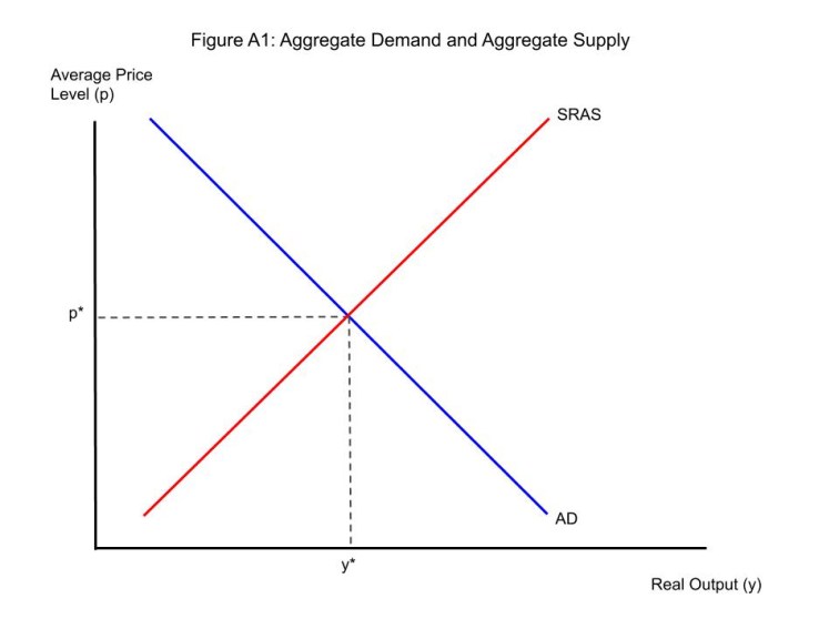
As usual, the intersection of the AD and SRAS curves endogenously determines the equilibrium average price level, p*, a nominal variable, and equilibrium real output, y*, a real variable.  Agents with rational expectations use this information to formulate expectations of the future price level; in this way, rational expectations are endogenous.  Thus, in a rational-expectations framework, the forecast errors that agents commit—and, yes, rational agents commit forecast errors; rational does not mean omniscient—are random with a mean of zero.  Put differently, because agents use all available information and interpret this information based on an accurate understanding of their complex economic environment (described by Figure A1, for example), agents do not err systematically—they learn from rather than repeat their mistakes.

More formally, then, according to the rational-expectations hypothesis, the equilibrium average price level at time t, p_t*, and its expectation at time t-1, which we write as E_t-1 [ p_t* ], are related in the following way.

p_t* = E_t-1 [ p_t* ] + ε_t

Where ε_t is a random, mean-zero error.  This is to say, the difference between the realization of the equilibrium average price level at time t, p_t*, and its expected value at time t-1, E_t-1 [ p_t* ], is a random, mean-zero error, ε_t, which, by definition, is unpredictable and, thus, not correctable at time t-1.  Moreover, because the policymaker does not generally have an informational advantage over other agents in a rational-expectations framework, ε_t is unpredictable from the policymaker’s perspective as well.  This means the policymaker cannot predictably (and, so, deliberately) affect y* (or any other real variable, including the unemployment rate).  This last point is crucial but not entirely obvious.  To appreciate it, consider a very simple mathematical example, where SRAS and AD are specified in the following ways.

SRAS:  y_t = b ( p_t  – E_t-1 [ p_t ] ) + η_t

AD:  y_t = m_t – p_t + ν_t

According to the SRAS specification, all else equal, real output is positively related to the average price level; thus, holding expectations constant (and, thus, exogenous), Phillips-curve trade-offs exist.  According to the AD specification, real output is negatively related to the average price level.  The variable m represents macroeconomic stabilization policy; so, an increase in m shifts AD to the right.  For concreteness, assume m represents the money supply (though it could represent, say, the level of government spending).  Finally, η_t and ν_t are, respectively, random, mean-zero, and independently distributed aggregate-supply and aggregate-demand shocks, which no one controls or anticipates.  For example, a realization of η_t may be an oil discovery; a realization of ν_t may be a payment innovation that reduces the transaction costs of monetary exchange.

Solving SRAS and AD simultaneously for the equilibrium level of real output,  y_t*, yields the following expression.

y_t* = [b(m_t – E_t-1 [ p_t ] ) + bν_t + η_t]/(1+b)

According to this expression, all else equal, the equilibrium level of real output is positively related to the money supply.  However, the crucial takeaway from the rational-expectations hypothesis is that all else is not equal, because expectations—in this case, E_t-1 [ p_t ]—are endogenous: at the same time the money supply is changed, agents use all available information—including the model illustrated in Figure A1 and specified by the mathematical expressions for SRAS and AD—to formulate their expectations of the policy outcome.  More specifically, to formulate expectations of the average price level in this case, agents solve SRAS and AD simultaneously for the equilibrium level of the average price level, p*, and, then, take expectations of it; doing so yields the following (endogenous) rational expectation of the average price level.

E_t-1 [ p_t ] = E_t-1 [ m_t ]

This expectation formulation essentially implies agents associate changes in the average price level with changes in the money supply, as they should given the structure of this standard model.  Thus, according to the rational-expectations hypothesis, the equilibrium level of real output, complete with endogenously determined expectations of the average price level, is described by the following expression.

_yt* = [b(m_t – E_t-1 [ m_t ] ) + bν_t + η_t]/(1+b)

This equilibrium level of real output is positively related to unexpected changes in the money supply, m_t – E_t-1 [ m_t ], demand shocks, ν_t, and supply shocks, η_t, none of which a policymaker controls.  Intuitively, because agents rationally expect the inflationary consequences of intentional changes in the money supply (or other macroeconomic-stabilization variables), agents preemptively adjust prevailing prices and wages in order to preserve their market-clearing levels in real terms.  The change in the money supply does not affect the economy’s real features, including the level of real output or its corresponding unemployment rate.  Thus, Phillips-curve trade-offs are fleeting events that policymakers cannot exploit.  This result is known as the policy-neutrality proposition.

Finally, a related proposition is the Lucas critique, which is attributed to Nobel laureate Robert Lucas.  According to this critique, policymakers cannot rely on existing empirical specifications of the economy—coefficient estimates in macro-econometric regression models, for example—in order to evaluate how new policy regimes would affect features of the economy such as, say, real output or unemployment.  This is because existing specifications of the economy are estimated based on past policy regimes.  When a new policy regime is implemented, agents reformulate expectations accordingly; existing specifications of the economy are no longer informative.  For example, concluding, based on existing empirical specifications of the economy, that a new, expansionary exchange-rate-targeting policy regime will decrease unemployment neglects the response of agents who will reformulate expectations consistent with the new policy regime.

Today, rational expectations is a benchmark framework against which economists compare and defend all other models of expectation formation (because there are other models of expectation formation).  Importantly, most economists accept that rational-expectation outcomes that occur in principle may not materialize in practice.  For example, most economists reason the classical dichotomy holds in the very long run, only.  Thus, macroeconomic stabilization policies, such as expansionary monetary policy during the recession in 2008, are not entirely useless at all times; the policy-neutrality proposition does not always hold.  Likewise, most economists reason that changes in policy that are consistent with the existing policy regime—a change in the short-term interest rate in a long-established inflation-targeting regime, for example—are not necessarily vulnerable to the Lucas critique.

References

Friedman, Milton.  1968.  “The role of monetary policy.”  American Economic Review, 58, (March): 1-17.

Keynes, John. M.  1936.  The General Theory of Employment, Interest, and Money.  New York: Harcourt, Brace and Company.

Phelps, Edmund. S.  1968.  “Money-wage dynamics and labor market equilibrium.”  Journal of Political Economy, 76 (July/August, Part 2): 678-711.

Phillips, Alban W.  1958.  “The relation between unemployment and the rate of change of money wage rates in the United Kingdom, 1861-1957.”  Economica, 25, no. 100: 283-299.

Turnovsky, Stephen J.  1984.  “Rational expectations and the theory of macroeconomic policy: An exposition of some of the issues.”  Journal of Economic Education, 94, no. 4: 1055–1084.