This blog post accompanies the spring-2019 season finale of SDPR Morning Macro, which airs on Monday, May 20.  Please watch and listen for us in the fall.  Keep in touch.  And thank you.

In February 1948, crowds filled Prague’s Old Square as Communist Czechoslovak Prime Minister Klement Gottwald announced the Communist Party of Czechoslovakia had successfully instigated a coup d’état.  By the summer of 1948, Gottwald was president; and Czechoslovakia sat behind the Iron Curtain of the Soviet Union (Steil 2018, p. 240).  By 1956, when Soviet premier Nikita Khrushchev announced to the free world, “We will bury you,” the communist threat to political and economic freedoms was palpable.  By then, economic growth in the Soviet Union far outpaced economic growth in the United States and Western Europe (even though Soviet economic growth heavily favored capital as opposed to consumer goods).  Because central planners could simply direct resources to meet production quotas, communism seemed destined to prevail.

Spoiler alert: communism did not prevail.

This weekend’s edition of the Wall Street Journal enticed readers to visit Prague’s Holesovice quarter, a once-gritty now-artsy neighborhood in the charming and sophisticated capital of the Czech Republic.  According to one Holesovice resident, “After the Velvet Revolution [in 1989] it was a mostly empty and dirty place. But that made good soil for creative businesses.”  Holesovice is a short metro ride from Wenceslas Square, where Soviet tanks crushed the Prague Spring in the summer of 1968.  This weekend’s Wall Street Journal piece—and my visit to Prague last summer—reminded me of the rich, intellectual history of macroeconomic growth theory and policy; a history shaped and, in some instances, inspired by the Cold War, when Soviet economic growth relied extensively on (forced) capital accumulation to grow output at exceptionally high annual rates.  As Soviet economies aggressively transformed capital and labor inputs into mostly industrial and military outputs, research into the sources of economic growth increasingly signaled the Soviet model was unsustainable.  Macroeconomists—of the non-Marxist sort—reasoned Khrushchev could not bury us, at least not in the long run.  The reasons why can teach us about the growth prospects of the current United States economy.

Macroeconomists have long puzzled over the sources of economic growth, which we measure as the average annual growth rate of output (or income) per capita over several decades—that is, the long run.  The consequences of economic growth are profound.  For example, an economy that sustains an economic growth rate of 1 percent annually would double output per capita about every 70 years; whereas an economy that sustains an economic growth rate of 2 percent annually would double output per capita about every 35 years.  Because most individuals would prefer, all else equal, to live in an economy in which the average standard of living doubles, say, twice in a lifetime instead of once in a lifetime, understanding economic growth—-including how macroeconomic policies shape it—-is very important.

By definition, economic growth is a dynamic process, because changes in output per capita occur over time.  It is helpful to think about output per capita (γ; output / population) at a moment in time as the product of labor productivity, labor hours per employee, the employment rate, and the labor-force participation rate, as follows.

γ = ρ × η × ε × λ

Where ρ is labor productivity (output / employee-labor hour), η is labor hours per employee, ε is the employment rate (employees / labor force), and λ is the labor-force participation rate (labor force / population).  This decomposition must be true based on how we define γ, ρ, η, ε, and λ.  By definition, then, output per capita (γ) must equal the product of the four terms on the right-hand side of the expression.  In Figure 1, I illustrate the log of United States output per capita (which I measure as real GDP per capita) since the Second World War.  In terms of the expression above, Figure 1 illustrates a measure of the natural logarithm of γ; thus, changes in this measure—revealed by slopes of lines tangent to Figure 1—represent growth rates of output per capita.

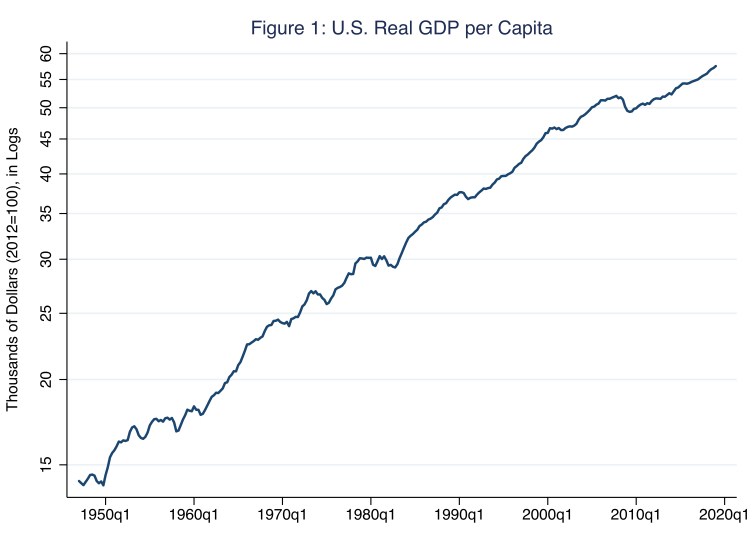
According to Figure 1, output per capita in, say, the last quarter of 2018, was $58,000 in year-2012 dollars.  Perhaps more importantly, from 1948 to 2018, output per capita grew on average at an annual rate of 2 percent; at this rate, the average standard of living in the United States—measured, in this case, by real GDP per capita—doubles every 35 years.  Visual inspection of Figure 1 reveals that output per capita includes a cyclical component that varies irregularly around a long-run trend such that output per capita occasionally exhibits relatively long-lived growth effects—persistent changes in the rate of growth (around trend growth of 2.0 percent annually in this case).  Thus, during the seventy-year period captured in Figure 1, annual growth in output per capita varied, at times substantially.  For example, in the decade since the Great Recession (from 2009 to 2018), output per capita in the United States grew on average at an annual rate of 1 percent; at this rate, the average standard of living doubles every 70 years.

Economic-growth rates matter—a lot.

If we want to know the principal sources of the growth rate of the standard of living, we need to consider the earlier expression, which specifies output per capita (γ) as the product of labor productivity (ρ), labor hours per employee (η), the employment rate (ε), and the labor-force participation rate (λ).  Mathematics—not macroeconomics—tells us that because output per capita is the product of these terms, the growth rate of output per capita—our measure of the growth rate of the standard of living—is, to a very close approximation, the sum of the growth rates of these terms, as follows.

growth rate of γ = growth rate of ρ + growth rate of η + growth rate of ε + growth rate of λ

So, the principal sources of the growth rate of the standard of living—notationally, the growth rate of γ on the left-hand side of the expression—are the growth rates of labor productivity (ρ), labor hours per employee (η), the employment rate (ε), and the labor-force participation rate (λ).  In Table 1, I report the average annual growth rates of γ, ρ, ε, and λ for various sample periods.  (I do not report the annual growth rate of labor hours per employee [η] because it varies relatively little; for example, for the last forty years, η has measured about 1800 hours, or about 52 weeks times about 35 hours per week.)

Table 1: Average Annual Growth in Output per Capita (γ) and Its Principal Sources

	γ	ρ	ε	λ
1960 – 2018	2.0%	2.0%	0.0%	0.1%
1960 – 1972	2.8%	2.8%	0.0%	0.1%
1973 – 1995	1.9%	1.5%	0.0%	0.4%
1996 – 2007	2.2%	2.7%	0.1%	– 0.1%
2009 – 2018	1.0%	1.3%	0.2%	– 0.5%

Notice, across each row, the average annual growth rate of output per capita (γ) equals, to a close approximation, the sum of the average annual growth rates of labor productivity (ρ), the employment rate (ε), and the labor-force participation rate (λ).  For example, consider the row associated with the sample period 2009 to 2018: the average annual growth rate of output per capita (γ) is 1.0 percent, which equals the average annual growth rate of labor productivity (ρ = 1.3 percent) plus the average annual growth rate of the employment rate (ε = 0.2 percent) plus the average annual growth rate of the labor-force participation rate (λ = – 0.5 percent).  To be sure, because of how we empirically define and measure these terms, this additive relationship is not perfect—consider, for example, the row associated with the sample period 1996 to 2007; nevertheless, the relationship is as close to truth as anything a macroeconomist encounters!

As Morning Macro devotees would expect, the average annual growth rates of output per capita (γ) and labor productivity (ρ)—columns two and three in Table 1—align over time because labor productivity is the most important source of output per capita.  For example, for the entire sample period of 1960 to 2018, the average annual growth rates of output per capita and labor productivity each equal 2.0 percent.  This alignment generally occurs because, in the long run, labor-market forces reflected in, say, the rates of job search and separation determine the (natural) employment rate (ε), while demographic forces largely determine the labor-force participation rate (λ).  Because labor-market and demographic forces change relatively slowly over time, these forces do not explain much of the change in output per capita.  Put differently, then, changes in labor productivity explain a large share of economic growth.  (For more on natural rate of unemployment, see the Morning Macro segment, “Separation Anxiety.”)

According to Table 1, the sample period 1960 to 1972 was a high-water mark for economic growth and, thus, labor productivity; output per capita (γ) and labor productivity (ρ) each grew on average 2.8 percent annually.  In contrast, the sample period 1973 to 1995 was a low-water mark; output per capita (γ) and labor productivity (ρ) grew on average 1.9 percent and 1.5 percent annually (while the labor-force participation rate grew on average 0.4 percent annually).  Since the recession that began in the first quarter of 2008, output per capita (γ) and labor productivity (ρ) have grown at alarmingly low rates of 1 and 1.3 percent, perhaps signaling a new low-water mark.

Clearly, labor productivity is an important source of economic growth; but, what determines labor productivity?  Consider the model of economic growth presented by Robert M. Solow (1956), in which output is a function of capital—physical and, potentially, human—and labor inputs.  Perfectly competitive firms in this model produce output using these inputs and available technology.  Thus, in this model, the quantity of capital per labor input and technology determine labor productivity.  Over time, increases in the quantity of capital and improvements in technology increase labor productivity, driving economic growth.  Specifically, saving—foregoing consumption—increases capital; and innovating improves technology.  Today, the Solow growth model is a standard feature of macroeconomic studies.

An important assumption of the model is that the production of output exhibits constant returns to scale in capital and labor: for example, doubling the quantities of capital and labor doubles the quantity of output.  This assumption is reasonable if gains from specialization are exhausted (so returns are not increasing) and inputs other than capital and labor are relatively unimportant (so returns are not decreasing).  A corollary of this assumption is that the production of output per labor input—that is, labor productivity—exhibits decreasing returns to scale in capital per labor input: for example, doubling the quantity of capital per labor input less than doubles the quantity of output per labor input.  This pattern of decreasing returns to scale is captured by the concave production function illustrated in Figure 2, where κ represents capital per labor input.

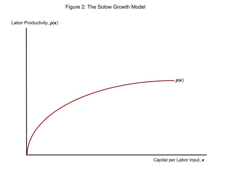
According to Figure 2, as the economy accumulates capital (by saving more), capital per labor input (κ) moves from left to right along the horizontal axis.  Consequently, labor productivity (ρ) rises along the vertical axis.  This pattern occurs because increasing the quantity of capital per labor input effectively equips each unit of labor with additional (productive) machinery and equipment, for example.  Nevertheless, because production exhibits decreasing returns to scale, labor productivity rises at a decreasing rate.  The upshot is that increasing the saving rate cannot increase the long-run growth rate of labor productivity; rather, increasing the saving rate can only increase the long-run level of labor productivity.  Put differently, given diminishing returns, accumulating capital is not an effective way to sustain economic growth.

Rather, the most effective way to sustain economic growth is to improve technology—the recipe, as it were, that transforms inputs (such as capital) into outputs.   In the context of Figure 2, technological improvements shift up the production function, ρ(κ); labor productivity increases even though the capital stock is fixed.  In effect, improving technology overcomes diminishing returns.  In practice, we refer to this technological force as total-factor productivity, which we define as a residual: the growth of labor productivity unaccounted for by the accumulation of capital or labor quality (aka, human capital).  Admittedly, total-factor productivity is a seemingly nebulous concept—the dark matter of macroeconomics; nevertheless, we can measure it.  Based on the careful work of John G. Fernald (2014), in Figure 3 I decompose the growth rate of United States labor productivity from 1948 to 1968 (from Prague coup to Prague Spring) into three sources: total-factor productivity (TFP), capital, and labor quality.

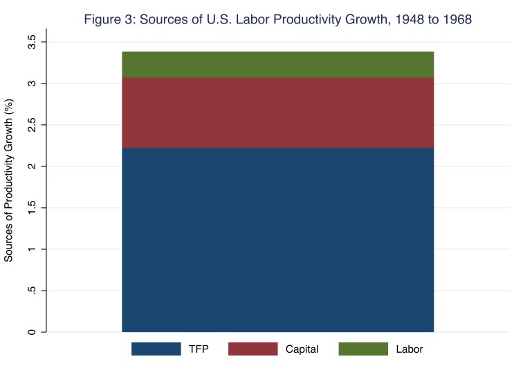
During the sample period 1948 to 1968, the growth rate of United States labor productivity averaged (an astounding) 3.4 percent annually; in Figure 3, 3.4 percentage points measure the combined height of the blue, red, and green bars.  Of these 3.4 percentage points, total-factor productivity accounted for 2.2 percentage points, or two thirds of the growth rate of labor productivity; capital accumulation and labor quality accounted for 0.9 and 0.3 percentage points, respectively.  So, absent the growth of total-factor productivity, during the sample period 1948 to 1968, the growth rate of United States labor productivity would have averaged (a not-very-astounding) 1.2 percent annually; put differently, absent the growth of total-factor productivity, Khrushchev may have buried us.  This general pattern of total-factor productivity driving economic growth persists to this day.  In Figure 4, I decompose the growth of U.S labor productivity since the Great Recession (from 2009 to 2018).

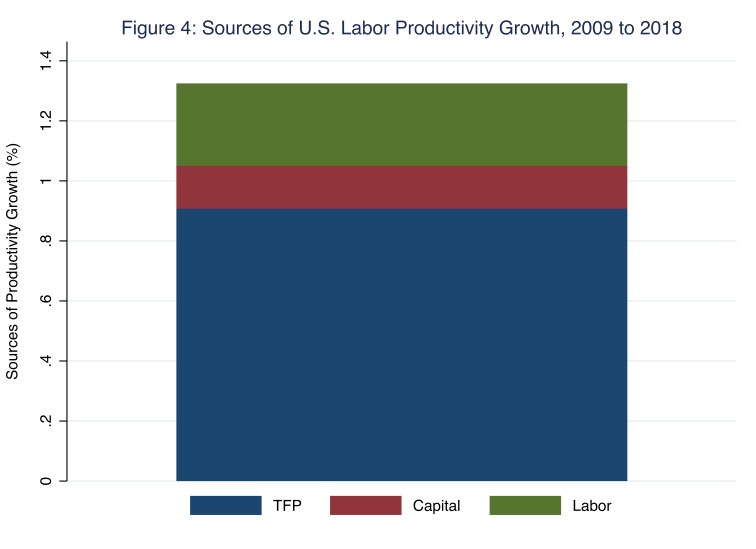
According to Figure 4, since the Great Recession, the growth rate of United States labor productivity has averaged (an underwhelming) 1.3 percent annually—the same 1.3 percent, incidentally, that I report in Table 1 in the last row of the column headed, ρ.  In any case, of these 1.3 percentage points, total-factor productivity accounted for 0.9 percentage points, or roughly two thirds of the growth rate of labor productivity; capital accumulation and labor quality accounted for 0.1 and 0.3 percentage points, respectively.  Essentially, then, the growth rate of United States labor productivity has averaged 1.3 percent annually since the Great Recession instead of 3.4 percent annually from 1948 to 1968 because total-factor productivity growth has averaged 0.9 percent instead of 2.2 percent, and because capital accumulation has averaged 0.1 percent instead of 0.9 percent.  (The growth in labor quality averaged 0.3 percent annually in both periods.)  Put another way, absent the growth of total-factor productivity, since the Great Recession the growth rate of United States labor productivity would have averaged (an even more underwhelming) 0.4 percent annually, at which rate the average standard of living would double about every 175 years.  In summary, economic growth is largely determined by labor productivity, which, in turn, is largely determined by total-factor productivity.

Generally speaking, innovative ways of transforming inputs into outputs drive total-factor productivity.  And, yes, Morning Macro devotees, specialization and exchange—free trade—is an innovative way of transforming inputs into outputs.  (For more on trade, see the Morning Macro segment, “Traitors.”)  Most economists reason that innovation is a largely endogenous process, an outcome of competitive interactions of firms maximizing shareholder value and operating in an economic environment that incentivizes activities that increase private and social returns.  Not surprisingly, then, total-factor productivity is most likely to grow in an economic system of sensibly regulated market capitalism, complete with specialization and exchange (including international trade), as opposed to centrally planned communism (where free enterprise and private property are prohibited).  To sustain high economic growth, a central planner must rely on capital accumulation (aka, capital deepening) to the point of repressing consumption.  And, even then, the returns to such a repressive, welfare-reducing approach eventually disappear.

Martin L. Weitzman (1970) characterized the Soviet challenge this way.

“A strategy of strong capital accumulation must be considerably less successful for the present relatively mature Soviet economy…Although a continuation on the same scale of a strategy of capital deepening can still yield growth rates which are high by Western standards, the days of relying almost exclusively on capital formation for producing 10 to 15 percent annual increases in industrial output would appear to be over” (p. 685).

Twenty years after Weitzman published his analysis of Soviet economic growth, on 9 November 1989, the Berlin Wall fell.  For weeks thereafter, crowds—including thousands of students—filled Prague’s Wenceslas Square, this time calling for the Communist Party of Czechoslovakia to end its monopoly grip on power; it did so in late November.  On 28 December, the Czechoslovak parliament, which by that time was mostly non-communist, elected as president, Václav Havel, the writer and former dissident.  With that, the Velvet Revolution closed the curtain on communist central planning in (then) Czechoslovakia.

Additional References

Fernald, John G.  2014.  “Productivity and potential output before, during, and after the Great Recession.”  Federal Reserve Bank of San Francisco Working Paper Series, Working Paper 2014-15, 1-50.

Solow, Robert M.  1959.  “A contribution to the theory of economic growth.”  The Quarterly Journal of Economics, 70, 65-94.

Steil, Benn.  2018.  The Marshall Plan: Dawn of the Cold War.  New York: Simon & Schuster.

Weitzman, Martin L.  1970.  “Soviet postwar economic growth and capital-labor substitution.”  American Economic Review, 60, 676-692.