This blog post accompanies the SDPR Morning Macro segment that airs on Monday, November 4.

Last Wednesday, the Federal Reserve’s Federal Open Market Committee (FOMC) cut its target range for the federal funds rate by a quarter of one percent; the range is now 1.5 to 1.75 percent.  This was the third rate cut since July.  The federal funds rate is the (interbank) rate that banks charge each other for bank reserves—inventories, essentially, that banks manage in order to generate earnings (by lending reserves to borrowers) and to maintain liquidity (by storing reserves for cash-seeking depositors).  To hit its federal funds rate target, the Fed manipulates the monetary base and, somewhat less precisely, the money supply.  (For more on the Federal Reserve System, the FOMC, and how the Fed’s trading desk manipulates the monetary base in order to keep the federal funds rate within the target range, see the Morning Macro segment, “Fed Up.”)  In Figure 1, I illustrate the quarterly average federal funds rate since 1960.

The federal funds rate earns an enormous amount of attention in the financial press, because the rate reflects the so-called stance of monetary policy: namely, expansionary (because output is below potential or inflation is below the Fed’s target rate) or contractionary (because output is above potential or inflation is above the Fed’s target rate).  For example, notice how the Fed dramatically lowered its target range for the federal funds rate to near zero—a most-expansionary monetary policy—around the start of the Great Recession (when output fell far below its potential while inflation fell below the Fed’s target rate).

In any case, setting and hitting targets for an overnight interbank lending rate is a tactical—that is, operational—feature of monetary policy.  Tactics are informed by goals and strategy.  And, in the case of the Federal Reserve System, the goal of monetary policy, ever since a 1977 amendment to the Federal Reserve Act, is to achieve a dual (Congressional) mandate of maximum employment (and, thus, output at or very near its potential) and stable prices (and, practically, low and stable inflation).  On January 29, 2012, the FOMC released its “Statement on Long-Run Goals and Monetary Policy Strategy,” in which the committee agreed to a single numerical inflation-target value of 2 percent based on the personal consumption expenditures price index; the agreement is sufficiently flexible so as to be consistent with the dual mandate.  

The difference between actual output and potential output—the level of output the economy would achieve if it were operating at full capacity—is what economists call the output gap; and, the difference between the actual inflation rate and the target inflation rate (of 2 percent) is what economists call the inflation gap.  Put differently, then, setting and hitting targets for an overnight interest rate is all about minding the gaps.  Generally speaking, a positive [negative] output gap reflects an economy that is operating above [below] its potential; all else equal, the appropriate tactical response in this case is for the Fed to raise [lower] its target range for the federal funds rate.  Similarly, a positive [negative] inflation gap reflects an economy in which the average price level is rising too quickly [slowly] relative to the Fed’s target inflation rate; again here, all else equal, the appropriate tactical response is for the Fed to raise [lower] its target range for the federal funds rate.

To evaluate whether the current stance of monetary policy is appropriate, mind the gaps.  In Figure 2, I illustrate the output gap, which I define as the difference between actual and potential output as a percentage of potential output; the latter is an estimate determined by the nonpartisan Congressional Budget Office.

In Figure 2, I include a blue reference line at the y-axis value of a zero output gap.  Where the actual output gap intersects the blue reference line, the economy is operating at full capacity; and, all else equal, the appropriate tactical response is for the Fed to set its target range for the federal funds rate at a neutral level—one that neither cyclically expands nor contracts aggregate demand.  Likewise, where the gap is above [below] the blue reference line, the economy is operating above [below] its potential; and, all else equal, the appropriate tactical response is for the Fed to raise [lower] its target range for the federal funds rate.  In the second quarter of 2019, the output gap was positive and equal to 0.83 percent of potential output.  Thus, the current output gap recommends a greater-than-neutral federal funds rate target range.  Hold that thought.

In Figure 3, I illustrate the inflation gap, which simply equals the actual inflation rate minus the Fed’s target inflation rate of 2 percent; here I measure the inflation rate based on the core personal consumption expenditures price index, the Fed’s preferred measure.

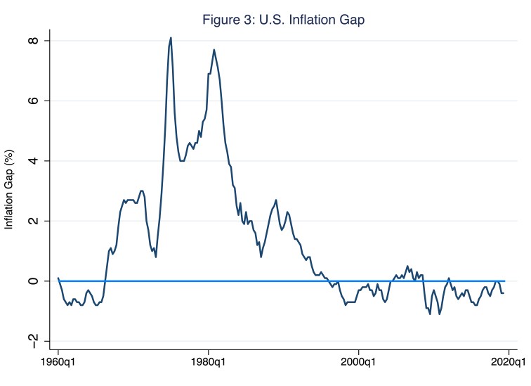
In Figure 3, I include a blue reference line at the y-axis value of a zero inflation gap.  Where the actual inflation gap intersects the blue reference line, the average price level is rising at a rate consistent with low and stable inflation; and, all else equal, the appropriate tactical response is for the Fed to set its target range for the federal funds rate at a neutral level.  Likewise, where the gap is above [below] the blue reference line, the average price level is rising too quickly [slowly] relative to the Fed’s target inflation rate; and, all else equal, the appropriate tactical response in this case is for the Fed to raise [lower] its target range for the federal funds rate.  In the second quarter of 2019, the inflation gap was equal to an annualized rate of negative 0.40 percent.  This is to say, in that quarter, the average price level rose at an annualized rate of 1.60 percent instead of the targeted 2.0 percent; or, put very differently (and somewhat intriguingly), the purchasing power of money fell too slowly relative to the Fed’s target inflation rate.  Thus, the current inflation gap recommends a less-than-neutral federal funds rate target range.

So the output gap is (slightly) positive while the inflation gap is (slightly) negative.  What’s a Fed to do?

Enter John Taylor.

Stanford economist John Taylor is best known among economists for his contributions to monetary theory and its implications for applied monetary policy.  Among Taylor’s many revolutionary accomplishments is the so-called Taylor rule, part of a large body of work in dynamic macroeconomic theory (complete with economic models with staggered wage and price setting and, thus, nominal rigidity).  Generally speaking, a Taylor rule essentially relates the central bank’s operational target (think, the federal funds rate) to the central bank’s goals (think, the output and inflation gaps).  The most common specification of this relationship is Taylor’s conveniently simple version, which I call Taylor rule 1.0, specified as the following:

i = r* + π + 0.5×(inflation gap) + 0.5×(output gap)

In this expression, the term i is the target federal funds rate; r* is the so-called natural (think, long-run) real rate of interest, and π is the rate of inflation.  The output and inflation gaps are those I defined and described above.  The weights on the gaps—in the specification above, the 0.5 multiplied times the inflation gap and the 0.5 multiplied times the output gap—reflect the central bank’s preferences for output and inflation stability (or, alternatively, the central bank’s aversion to output and inflation variability). In the case of the Fed, we presume these preferences (or aversions) are informed by the dual mandate.  So, for example, according to the specification above, if the actual rate of inflation is equal to 2 percent (and so the inflation gap is zero) and output is equal to its potential (and so the output gap is zero), then the (neutral) federal funds rate (i) should be equal to r* + π or about 4.0 percent, assuming (however wishfully) that the natural real rate of interest (r*) is 2 percent, the subject of a future Morning Macro segment.  Positive [Negative] output or inflation gaps raise [lower] the federal funds rate target above [below] 4.0 percent accordingly.  In Figure 4, I illustrate a federal-funds rate target informed by Taylor rule 1.0.

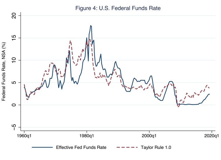
In Figure 4, the blue line is the actual federal funds rate, which I reproduce from Figure 1; the red, dashed line is the federal funds rate target that Taylor rule 1.0 recommends based on the output- and inflation-gap inputs I chose.  Notice how well the rule fits the actual rate, particularly since about the late 1990s—the beginning of a de-facto inflation targeting framework for U.S. monetary policy (Santos 2012).  Indeed, in a few cases in the past when the rule deviated dramatically from the actual rate, monetary-policy outcomes were not ideal: consider, for example, the dramatic deviation during the 1970s and early 1980s, during the so-called Great Inflation.  (In fairness to the Fed, alternative, more-favorable interpretations of monetary policy during this period abound; see, for example, Orphanides [2003]).  Since the Great Recession, the Taylor rule has recommended a relatively tight monetary policy—one that would have kept the federal funds rate higher than the actual rates (the blue line) that the Fed delivered.  This is to say, according to the Taylor rule, currently, the positive output gap and the negative inflation gap recommend a federal funds rate target range that is higher than the range of 1.5 to 1.75 percent that we now observe.

Of course, no single specification of a policy rule is generally accepted by all economists.  Moreover, how we measure the output gap, the inflation gap, and the natural real rate of interest (r*), can matter a great deal.  For example, should we use the central bank’s forecast of each gap instead of the actual gap?  How do we measure r*?  And how do we account for the central bank’s anticipation and preemptive responses to other potential macroeconomic shocks for which a Taylor rule may not adequately account?  These questions are important; nevertheless, most Taylor rule specifications that tightly fit the actual federal funds rate in the two decades before the Great Recession recommend higher rates today.  Consider, for example, the fit since 1999 of another popular version of the Taylor rule—one that former Chairman Bernanke proposed in place of Taylor rule 1.0—specified as the following:

i = r* + π + 0.5×(inflation gap) + 1.0×(output gap)

This expression, which I call Taylor rule 2.0, differs from Taylor rule 1.0 in only one way: the weight on the output gap is 1.0 instead of 0.5; intuitively, compared to the central bank informed by Taylor rule 1.0, the central bank informed by Taylor rule 2.0 more strongly prefers output stability.  In Figure 5, I illustrate a federal-funds rate target informed by Taylor rule 2.0

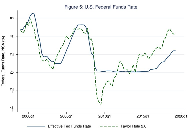
According to Figure 5, from 1999 to 2015, the only time that actual Fed tactics differed from those the rule recommends was immediately after the Great Recession, when the Fed chose (rightly, I would argue) not to impose negative interbank rates.  However, since about 2015, Taylor rule 2.0 has recommended a higher federal funds rate; today that rate would fall within a quarterly average range of 4 to 4.25 percent.  Even if we argue that r* has fallen since the Great Recession to (an unprecedentedly low) 0 percent, Taylor rule 2.0 recommends a current quarterly average target range of 2 to 2.25 percent, fifty basis points above the Fed’s current target range.  Perhaps it is no wonder the Fed indicated last week that it would not lower its target range again unless new data on output and inflation gaps  were to suggest otherwise; to be sure, this policy stance is broadly consistent with Taylor rule 2.0.

So, then, the Fed should unquestionably follow a Taylor rule?  No.

Taylor rules are too simple, no matter the complex models from which we derive such rules.  Simple algebraic expressions such as Taylor rule 1.0 or 2.0 cannot capture the intangible nuances of informed judgements—about the present and the future—required to implement optimal monetary policy.  Granted, specifying and estimating policy rules is a highly productive way to model, simulate, understand, and, thus, implement monetary policy.  Analyzing disparities—as I have done in this blog post—between reasonably specified Taylor rules and actual federal funds target ranges is instructive and, thus, worthwhile.  Nevertheless, the idea that Taylor rules—those recommended by John Taylor or otherwise—suitably prescribe monetary policy is, in my view, a bridge too far.  In practice, algorithmic rules do not outperform well-informed, rational, and apolitical discretionary monetary policy—the outcomes of FOMC deliberations, essentially.  

References

Orphanides, Athanasios.  2003.  “The Quest for Prosperity without Inflation.” Journal of Monetary Economics, 50 (3): 633–663

Santos, Joseph M.  (2012)  “What’s so special about inflation targeting? A comparative analysis of recent Canadian and US monetary policy frameworks.”  American Review of Canadian Studies, 42, 257-275